Fluvial knickpoints on the Roan Plateau (MATLAB)#
Authors#
Wolfgang Schwanghart, University of Potsdam, FU Berlin (homepage, GitHub)
William S. Kearney, University of Potsdam
This notebook is licensed under CC-BY 4.0.
Highlighted References#
Schwanghart, W. and Scherler, D.: Divide mobility controls knickpoint migration on the Roan Plateau (Colorado, USA), Geology, 48, 698–702, https://doi.org/10.1130/G47054.1, 2020.
Audience#
This is the MATLAB script presented at the EGU webinar: Topographic analysis using TopoToolbox in MATLAB and Python. It is suitable for beginners and more advanced users of TopoToolbox.
Introduction#
Fluvial knickpoints, here defined as sharp convexities along river profiles, are important topographic markers indicative of changes in base level of rivers, rock uplift, variations in rock resistance or processes leading to rapid changes in discharge. Here we revisit the Parachute Creek catchment, a basin of the Roan Plateau, that experienced a base level change as the Colorado River rapidly incised 8 Myrs ago (Berlin and Anderson, 2007, Schwanghart and Scherler, 2020). The catchment is steeply dissected by canyons whose heads feature remarkable knickpoints. In this exercise, we will learn to automatically detect these features in longitudinal river profiles, and how they can be used to estimate stream power parameters. To this end, we will use the stream-power incision model to simulate the upstream migration of knickpoints.
Dependencies#
To run this code, you’ll just need TopoToolbox including its required toolboxes. Some functions will need the Statistics and Machine Learning Toolbox.
Load the DEM#
We will use readopentopo to download the DEM.
[1]:
%% Read DEM
DEM = readopentopo('extent',[-108.3168 -107.8432  39.3843  39.6960],...
    'demtype','COP30');
[1]:
-------------------------------------
readopentopo process:
DEM type: COP30
API url: https://portal.opentopography.org/API/globaldem?
    "Local file name: "    "/home/runner/.cache/topotoolbox/OpenTopo_39.3843_39.696_-108.3168_-107.8432_COP30.tif"
Area: 1.4e+03 sqkm
-------------------------------------
Starting download: 02-Jun-2026 12:55:04
Download finished: 02-Jun-2026 12:55:16
Reading DEM: 02-Jun-2026 12:55:16

The downloaded DEM is not in a projected coordinate system.
Make sure to project the DEM using GRIDobj/project or
GRIDobj/reproject2utm.

DEM read: 02-Jun-2026 12:55:17
Done: 02-Jun-2026 12:55:17
-------------------------------------
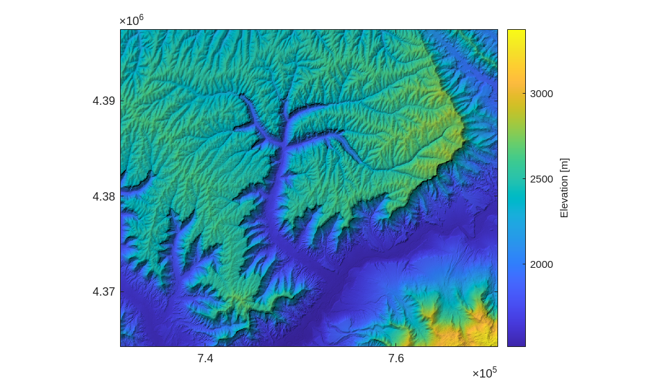
The DEM comes in geographic coordinates, hence, we will need to transform it to a projected coordinate system. reproject2utm identifies the right UTM-zone and uses bilinear grayvalue interpolation by default. The function GRIDobj/project gives you more control on the projection used. The transformation will produce regions of NaNs along the DEM edges. The function largestinscribed removes these nans and returns a DEM without NaNs.
[2]:
DEM = reproject2utm(DEM,30);
DEM = largestinscribedgrid(DEM);
imageschs(DEM,'colorbarylabel','Elevation [m]')
[2]:
Preparing the stream network#
We now take the DEM to derive the flow and stream network.
[3]:
%% Extracting the flow and stream network
FD = FLOWobj(DEM);
S  = STREAMobj(FD,minarea = 1000);
We are only interested in the network of the Parachute Creek. The tricky thing will be to programmatically determine this stream network. Here, we use klargestconncomps and removeedgeeffects, but below you’ll find commented code for interactive or semiautomated approaches, too.
[4]:
% Extract the Roan catchment
% This is the easiest and automated way to get the Parachute creek but
% I have listed a few other options below.
S  = klargestconncomps(S,1);
S  = removeedgeeffects(S,FD);
S  = klargestconncomps(S);

% Different ways to extract the Roan catchment
% S  = modify(S,'interactive','polyselect');
% S  = modify(S,'interactive','outletselect');

% Or, if you know the outlet location
% ix = 795228;
% S = modify(S,'upstreamto',ix);

% Or, if we know the approximate location
% x = 752545;
% y = 4371660;
% [x,y,ix] = snap2stream(S,x,y);
% S = modify(S,'upstreamto',ix);
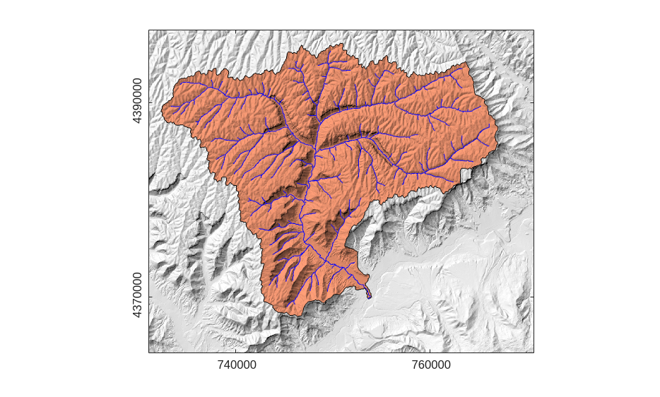
Let’s create a map, to make sure that we have correctly identified the basin.
[5]:
D = drainagebasins(FD,S);
GT = GRIDobj2geotable(D);
figure
imageschs(DEM,D>0,'truecolor',[1.0  0.62  0.47],'colorbar',false,...
    'ticklabels','nice')
hold on
mapshow(GT,'FaceColor','none','EdgeColor','k')
plot(S,'b')
[5]:
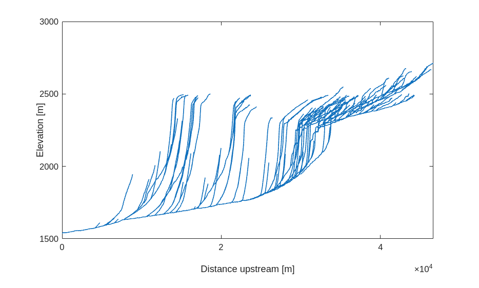
Plot the longitudinal river profile#
In a next step, we plot the river profile. You’ll notice that the river profiles feature several knickpoints upstream of which the rivers have quite low gradients.
[6]:
figure
plotdz(S,DEM)
[6]:
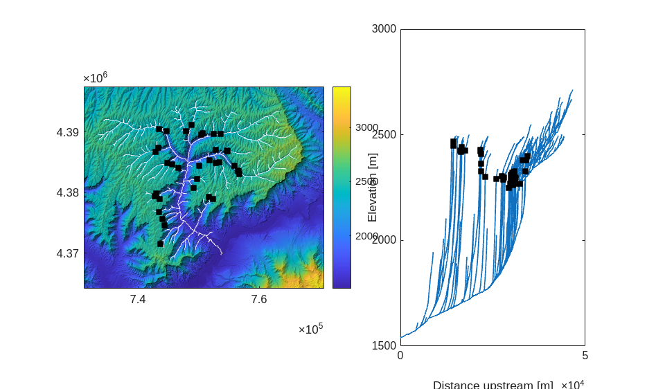
Identify knickpoints#
To identify the knickpoints, we use knickpointfinder, a function to automatically identify knickpoints in river profiles. Critical for knickpoint identification is setting an appropriate tolerance. The steep incision of the canyons allows us to set a fairly high tolerance value of 100 m
[7]:
[zs,kp] = knickpointfinder(S,DEM,'tol',100,'split',false,'plot',false);
[7]:
02-Jun-2026 12:55:21 -- Starting
02-Jun-2026 12:55:21 -- Iteration: 1, 1 knickpoints, max dz: 296.5237
02-Jun-2026 12:55:21 -- Iteration: 2, 2 knickpoints, max dz: 289.0972
02-Jun-2026 12:55:21 -- Iteration: 3, 3 knickpoints, max dz: 269.7761
02-Jun-2026 12:55:21 -- Iteration: 4, 4 knickpoints, max dz: 261.6294
02-Jun-2026 12:55:21 -- Iteration: 5, 5 knickpoints, max dz: 248.4626
02-Jun-2026 12:55:21 -- Iteration: 6, 6 knickpoints, max dz: 248.2458
02-Jun-2026 12:55:21 -- Iteration: 7, 7 knickpoints, max dz: 246.877
02-Jun-2026 12:55:21 -- Iteration: 8, 8 knickpoints, max dz: 246.3699
02-Jun-2026 12:55:21 -- Iteration: 9, 9 knickpoints, max dz: 244.8636
02-Jun-2026 12:55:21 -- Iteration: 10, 10 knickpoints, max dz: 239.9705
02-Jun-2026 12:55:21 -- Iteration: 11, 11 knickpoints, max dz: 237.873
02-Jun-2026 12:55:21 -- Iteration: 12, 12 knickpoints, max dz: 237.0083
02-Jun-2026 12:55:21 -- Iteration: 13, 13 knickpoints, max dz: 226.4376
02-Jun-2026 12:55:21 -- Iteration: 14, 14 knickpoints, max dz: 220.0303
02-Jun-2026 12:55:21 -- Iteration: 15, 15 knickpoints, max dz: 219.6909
02-Jun-2026 12:55:21 -- Iteration: 16, 16 knickpoints, max dz: 219.6826
02-Jun-2026 12:55:21 -- Iteration: 17, 17 knickpoints, max dz: 214.2446
02-Jun-2026 12:55:21 -- Iteration: 18, 18 knickpoints, max dz: 212.9622
02-Jun-2026 12:55:21 -- Iteration: 19, 19 knickpoints, max dz: 210.7898
02-Jun-2026 12:55:21 -- Iteration: 20, 20 knickpoints, max dz: 197.6343
02-Jun-2026 12:55:21 -- Iteration: 21, 21 knickpoints, max dz: 194.3284
02-Jun-2026 12:55:22 -- Iteration: 22, 22 knickpoints, max dz: 188.2834
02-Jun-2026 12:55:22 -- Iteration: 23, 23 knickpoints, max dz: 178.8977
02-Jun-2026 12:55:22 -- Iteration: 24, 24 knickpoints, max dz: 177.3721
02-Jun-2026 12:55:22 -- Iteration: 25, 25 knickpoints, max dz: 171.354
02-Jun-2026 12:55:22 -- Iteration: 26, 26 knickpoints, max dz: 149.8694
02-Jun-2026 12:55:22 -- Iteration: 27, 27 knickpoints, max dz: 146.9287
02-Jun-2026 12:55:22 -- Iteration: 28, 28 knickpoints, max dz: 146.4023
02-Jun-2026 12:55:22 -- Iteration: 29, 29 knickpoints, max dz: 140.0247
02-Jun-2026 12:55:22 -- Iteration: 30, 30 knickpoints, max dz: 138.7908
02-Jun-2026 12:55:22 -- Iteration: 31, 31 knickpoints, max dz: 137.0164
02-Jun-2026 12:55:22 -- Iteration: 32, 32 knickpoints, max dz: 127.5066
02-Jun-2026 12:55:22 -- Iteration: 33, 33 knickpoints, max dz: 107.1763
02-Jun-2026 12:55:22 -- Iteration: 34, 34 knickpoints, max dz: 105.6655
02-Jun-2026 12:55:22 -- Iteration: 35, 35 knickpoints, max dz: 101.9216
02-Jun-2026 12:55:22 -- Iteration: 36, 36 knickpoints, max dz: 100.384
Let’s plot the results.
[8]:
figure
subplot(1,5,1:3)
imageschs(DEM)
hold on
plot(S,'w')
plot(kp.x,kp.y,'sk','MarkerFaceColor','k')
subplot(1,5,[4 5])
plotdz(S,DEM)
hold on
plot(kp.distance,kp.z,'sk','MarkerFaceColor','k')
[8]:
Chi analysis#
The chi transformation is predicated on the stream-power incision model. The transformation is an integration of the inverse of upstream areas in upstream direction and thereby creates a new distance measure that linearizes the river profile (Perron and Royden 2013). We now calculate the chi transformation of the Parachute Creek using the function chitransform with an mn-ratio of 0.45 and a reference area of 1 sqkm. At a later stage, we will refine the mn-ratio.
[9]:
A = flowacc(FD);
c = chitransform(S,A,'a0',1e6,'mn',0.45);
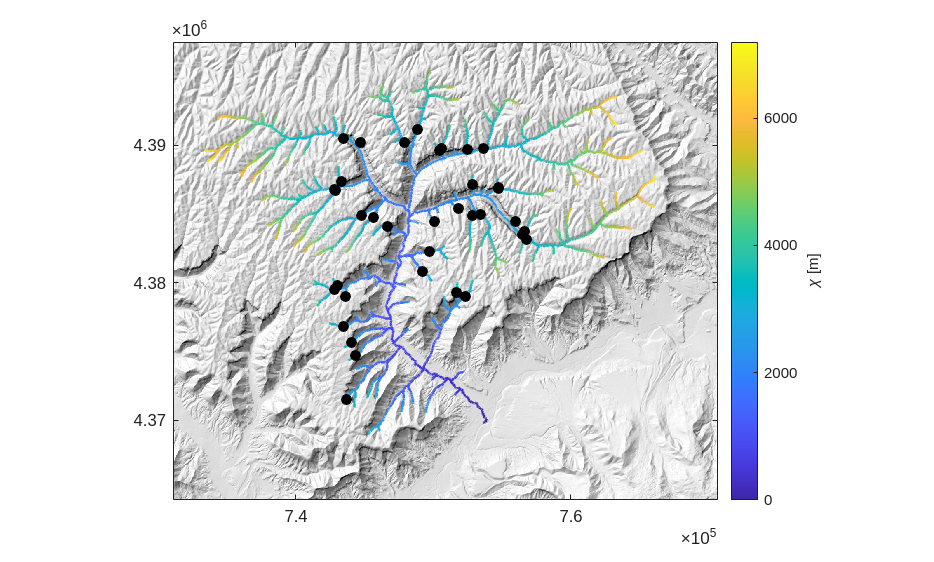
We then plot the results as a map. This map that is referred to chi map (Willett et al. 2014).
[10]:
figure
imageschs(DEM,'colormap',[1 1 1],'colorbar',false);
hold on
plotc(S,c)
plot(kp.x,kp.y,'ok','MarkerFaceColor','k')
h = colorbar;
h.Label.String = '\chi [m]';
[10]:
Modelling spatial patterns of knickpoints using PPS#
We will now use the PPS-class to analyze and visualize the knickpoints. PPS means Point Pattern on Stream networks and is a simple data class that contains the stream network (stored as STREAMobj) and the locations of the points.
[11]:
P = PPS(S,'PP',kp.IXgrid,'z',DEM);
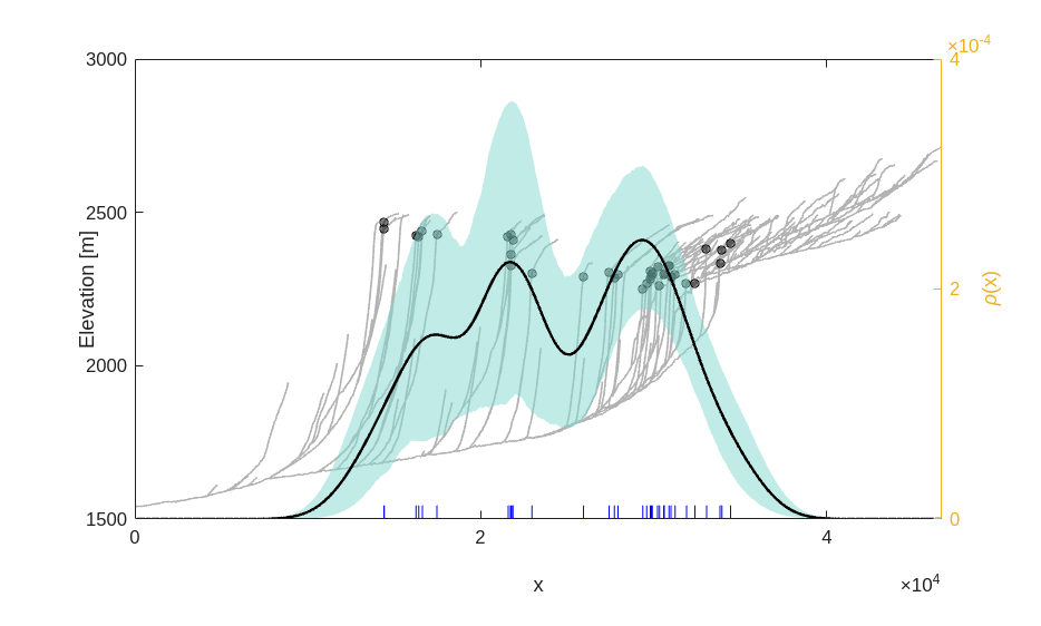
P is now an instance of the PPS class. For convenience, it also let’s you store river elevations. That’s why we added the DEM as z-property. We will now plot distance versus elevations of both the stream network using plotdz. In addition, we add a second axis. We will use this axis to plot a nonparametric dependence estimate using PPS/rhohat. The function returns a wiggly line that indicates the expected density of points for a given distance. You will notice that the points spread over a fairly large distance ranging between 10 to 35 km from the outlet.
[12]:
figure
plotdz(P,'colordata','k')
yyaxis right
rhohat(P)
[12]:
We now do the same, but this time, we use chi rather than the distance.
[13]:
figure
plotdz(P,'distance',c,'colordata','k')
yyaxis right
rhohat(P,'cov',c,'name','\chi')
xlabel('\chi [m]')
[13]:
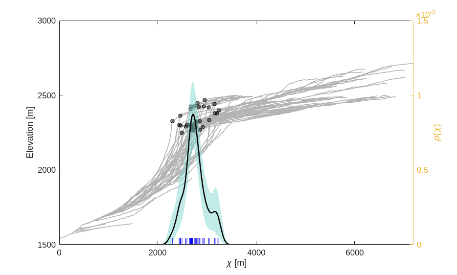
The stream profiles collapse to a dense set of lines and the knickpoints cluster in a narrow range of chi. This provides strong evidence that the knickpoints eminated from a common signal, i.e. the base level drop at the catchment outlet.
Modelling the knickpoint locations in time#
PPS features a function to retrieve stream-power parameters from the distribution of knickpoints. It is called mnoptimkp because the main purpose is to determine an optimal mn-ratio based on knickpoint locations. The function features several options and we encourage you to take a closer look at the help of the function. The best approach, but also one that is probably not working well if your data is broadly scattered in chi space, is provided by the method deviance. The approach fits a second-order loglinear model of the point density. The parameters of this fit yields some helpful information if you provide additional information on the onset of knickpoint migration (here 8 Myrs ago) and the uncertainty of this estimate (here we set an uncertainty of 1 Myrs).
[14]:
results = mnoptimkp(P,FD,"method","deviance","t",8e6,"sigmat",1e6);
results
[14]:
results = struct with fields:
        mn: 0.4400
       chi: [10284x1 double]
    chifun: @(mn)chitransform(P.S,a,'mn',mn,'a0',options.a0)
       mdl: [1x1 GeneralizedLinearModel]
       int: [10284x1 double]
    chimax: 2.8864e+03
         K: 8.2608e-07
    Ksigma: 1.0383e-07
      Kint: [6.2259e-07 1.0296e-06]
       tau: [10284x1 double]
    tauint: [10284x2 double]
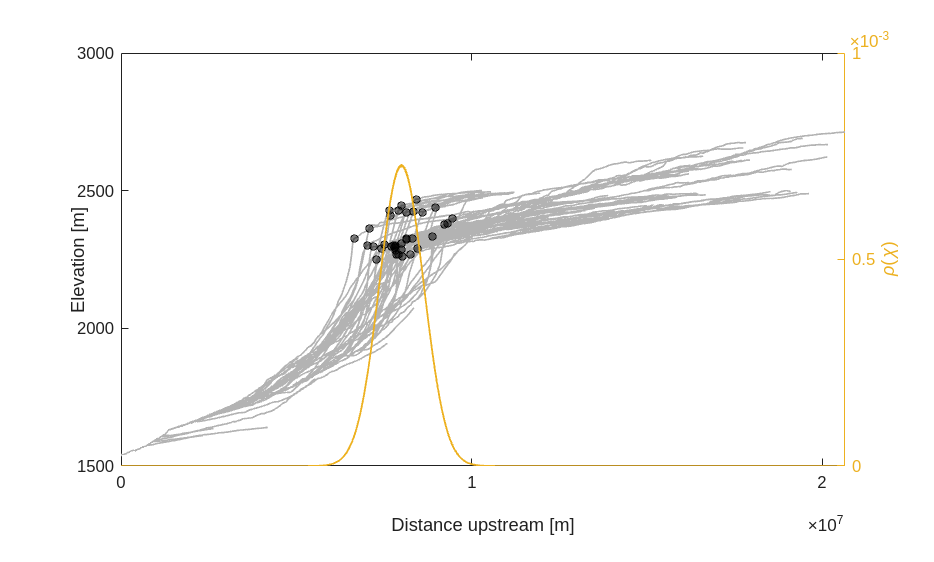
You will recognize the meaning of some of the fields of the structure array results. For example, there is an optimal mn-ratio, as well as a node-attribute list of chi values. The node-attribute list results.int gives you the modelled density of knickpoints and tau translates chi into a time based on an fitted value of K. Interestingly, the optimal mn-ratio is very close to the commonly used value of 0.45.
[15]:
figure
plotdz(P,'distance',results.tau,'colordata','k')
yyaxis right
plotdz(S,results.int,'distance',results.tau)
ylabel('\rho(\chi)')
[15]:
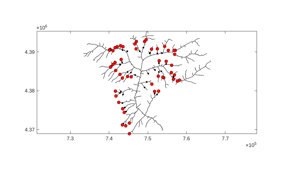
Dynamic plot of knickpoint migration#
Finally, let’s make a dynamic plot that shows how the knickpoints migrated upstream. This shows that knickpoint celerity sharply reduces once knickpoints enter tributaries with small catchment areas.
[16]:
t = (0:0.01:10) *1e6;

figure
plot(P);
axis equal
hold on
for r = 1:numel(t)
    [x,y] = getlocation(S,t(r),"value",results.tau,"output","xy");
    if r == 1
        h = plot(x,y,'ok','MarkerFaceColor','r');
    else
        h.XData = x;
        h.YData = y;
    end
    pause(0.01)
end
[16]:
References and Additional Information#
Berlin, M. M. and Anderson, R. S.: Modeling of knickpoint retreat on the Roan Plateau, western Colorado, Journal of Geophysical Research: Earth Surface, 112, https://doi.org/10.1029/2006JF000553, 2007.
Perron, J. T. and Royden, L.: An integral approach to bedrock river profile analysis, Earth Surf. Process. Landforms, 38, 570–576, https://doi.org/10.1002/esp.3302, 2013.
Willett, S. D., McCoy, S. W., Perron, J. T., Goren, L., and Chen, C.-Y.: Dynamic Reorganization of River Basins, Science, 343, 1248765, https://doi.org/10.1126/science.1248765, 2014.