Smoothing river profiles (MATLAB)#

Authors#

Wolfgang Schwanghart, University of Potsdam, (homepage, GitHub)

This notebook is licensed under CC-BY 4.0.

Highlighted References#

Schwanghart, W., Scherler, D., 2017. Bumps in river profiles: uncertainty assessment and smoothing using quantile regression techniques. Earth Surface Dynamics, 5, 821-839. [DOI: 10.5194/esurf-5-821-2017]

Audience#

For beginners and more advanced users of TopoToolbox interested in the analysis of longitudinal river profiles.

Introduction#

If you work with river profiles derived from global, medium-resolution DEMs, you will notice that these profiles have quite some scatter, depicting river profiles as lines that go up and down. Of course, river elevations should monotoneously decrease when going downstream, and these excursion are mostly errors and artefacts that can be attributed to variable reasons. Among these reasons are data acquisition errors, resolution effects, and actual features that obstruct the view on the river such as bridges and culverts. Here, we will learn how to process river profiles so that their elevations are smoothed and are strictly decreasing. This can be very helpful, if you preprocess DEMs for hydraulic models (e.g. Bricker et al. 2016).

Dependencies#

To run this code, you’ll need the Optimization Toolbox together with the other dependencies required by TopoToolbox.

Calculating the river profile#

Before we start, let’s download a good example. We are going to use the Taiwan DEM which is part of the lightweight repository for DEM examples for TopoToolbox.

[1]:

% Download the example using readexample
DEM = readexample('taiwan');

In a second step, we’ll derive the flow network, the stream network, and the longest river in Taiwan. If I am not mistaken, this river is called Zhuo Shui Xi.

[2]:

FD  = FLOWobj(DEM);
S   = STREAMobj(FD,'minarea',1000);
S   = klargestconncomps(trunk(S));
[lat,lon] = STREAMobj2latlon(S);
geoplot(lat,lon)

[2]:

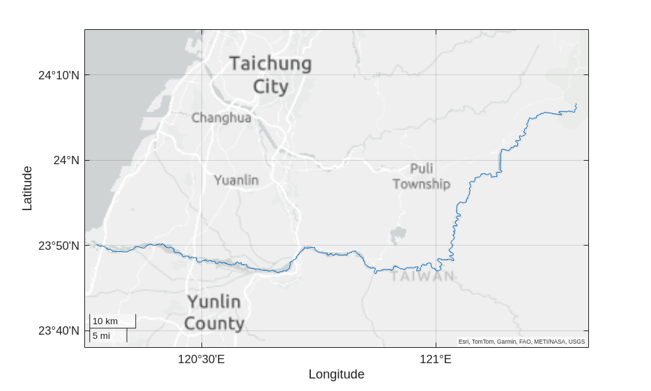
Now let’s plot the profile of the river.

[3]:

figure
plotdz(S,DEM,'dunit','km')

[3]:

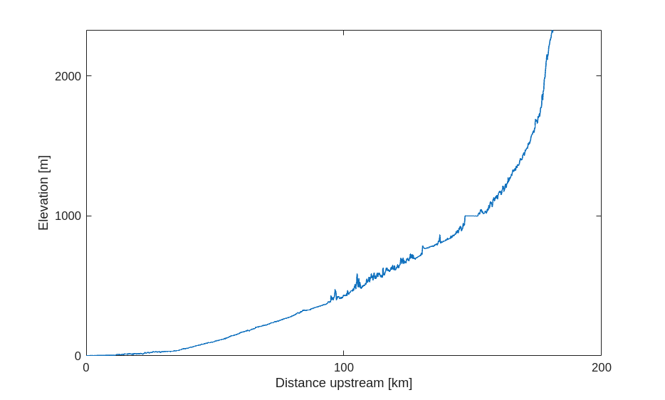
As you can see, there are quite some bumps along the river profile. In particular, there seems to be quite some variability between 100 and 130 km upstream distance. Why is this the case? Let’s plot a swath profile of the DEM along the river. Here, the width of the swath is 2000 m.

[4]:

SW = STREAMobj2SWATHobj(S,DEM,'width',2000);
figure
plotdz(SW)
hold on
h = plotdz(S,DEM,'color',ttclr('river'));
h.DisplayName = 'River profile';

[4]:

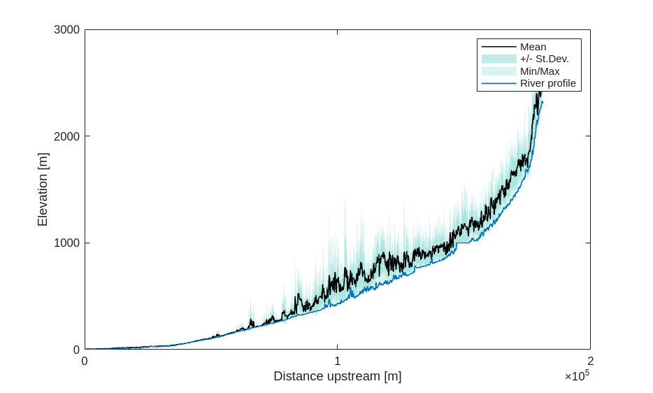
So, apparently, much of the variability along the river profile is related to a quite steep landscape left and right to the river, a problem that we frequently see in mountainous areas.

Removing bumps from the river profile#

Now let’s process the river profile so that we get rid of all the bumps. There are different STREAMobj methods to do this: crs, crslin, quantcarve and imposemin. In addition - and we’ll start with this one - there is flood filling, the most standard approach available in any GIS. We are now going to plot most of these to see their effects. In our plot, we will zoom into the the river profile to see more details.

[5]:

zf = getnal(S,fillsinks(DEM)); % Sink filling
zc = imposemin(S,getnal(S,DEM)); % Carving (or minima imposition)
zqc = quantcarve(S,DEM,0.3,"split",0);   % Quantile carving along the 20th percentile

% Some plotting parameters
dunit = 'km';

figure
h = plotdz(S,DEM,"dunit",dunit,"color",[.7 .7 .7]);
hold on
h(2) = plotdz(S,zf,"dunit",dunit);
h(3) = plotdz(S,zc,"dunit",dunit);
h(4) = plotdz(S,zqc,"dunit",dunit);
legend(h,"Original profile","Filling","Carving","Quantile carving",'Location','northwest');
xlim([100 130])

[5]:

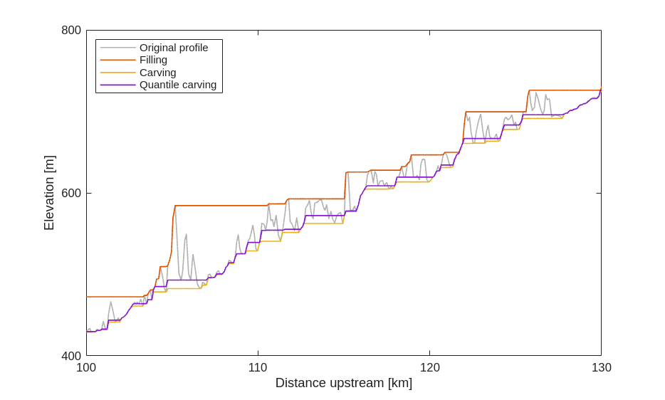
The different methods lead to vastly different results. The profile preprocessed using filling runs along the maxima of the profile, whereas the one obtained from carving runs along the minima. Quantile carving runs between both, so that, conditional on stream distance, 30% of the profile elevations lie below and 70% above the modelled profile. Obviously, both the shape of the filled and carved profiles is most affected by outliers in the data. This is certainly not something that we want.

So, let’s take a closer look at quantile carving. What this method does could be considered to be a isotonic quantile regression (also I was not aware of this method when developing quantcarve). An isotonic regression is a nonparametric method to determine an optimal (usually in terms of least squares), free-form trend through some data whereas the direction (increasing or decreasing) of the trend is determined beforehand. Quantcarve optimizes the curve so that the curve runs freely along some specified quantile. Let’s take a look at different quantiles.

[6]:

dunit = 'km';
figure
h = plotdz(S,DEM,"dunit",dunit,"color",[.7 .7 .7]);
legend("Location","northwest")
h.DisplayName = 'Original profile';
hold on
clr = num2rgb(1:9);
for r = 1:9
    zqc = quantcarve(S,DEM,r*0.1,"split",0);
    h(r+1) = plotdz(S,zqc,"dunit",dunit,"color",clr(r,:));
    h(r+1).DisplayName = [num2str(r*0.1*100) 'th percentile'];
end
hold off
xlim([100 130])

[6]:

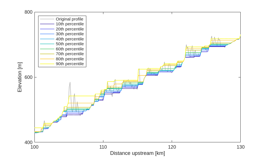
So, quantile carving represents a continuous transition between the two extremes, filling and carving, and it is up to you to determine which value of the quantile \(\tau\) is the best. My experience is that lower values between 0.1 and 0.3 usually match true elevations best.

Smoothing the river profile and removing bumps#

All profiles, whether they have been derived by filling, carving, or quantile carving have one thing in common. They all produce profiles that have plenty of sharp drops. Between those, river elevations are often constant. The final profile thus resembles an irregular staircase. And while this may be a good representation for some mountain streams with step-pool sequences, this shape is likely not representive of larger rivers. This is were the function crs comes in. The function name stands for constrained regularized smoothing. It resembles quantcarve but adds smoothing which is determined by another parameter, K. Let’s try it out:

[7]:

dunit = 'km';
figure
h = plotdz(S,DEM,"dunit",dunit,"color",[.7 .7 .7]);
legend("Location","northwest")
h.DisplayName = 'Original profile';
hold on
numExperiments = 5;
clr = num2rgb(1:numExperiments);
K   = [1 5 10 20 100];
for r = 1:numExperiments
    zs = crs(S,DEM,"tau",0.2,"K",K(r),"split",0);
    h(r+1) = plotdz(S,zs,"dunit",dunit,"color",clr(r,:));
    h(r+1).DisplayName = ['K = ' num2str(K(r))];
end
hold off
xlim([100 130])

[7]:

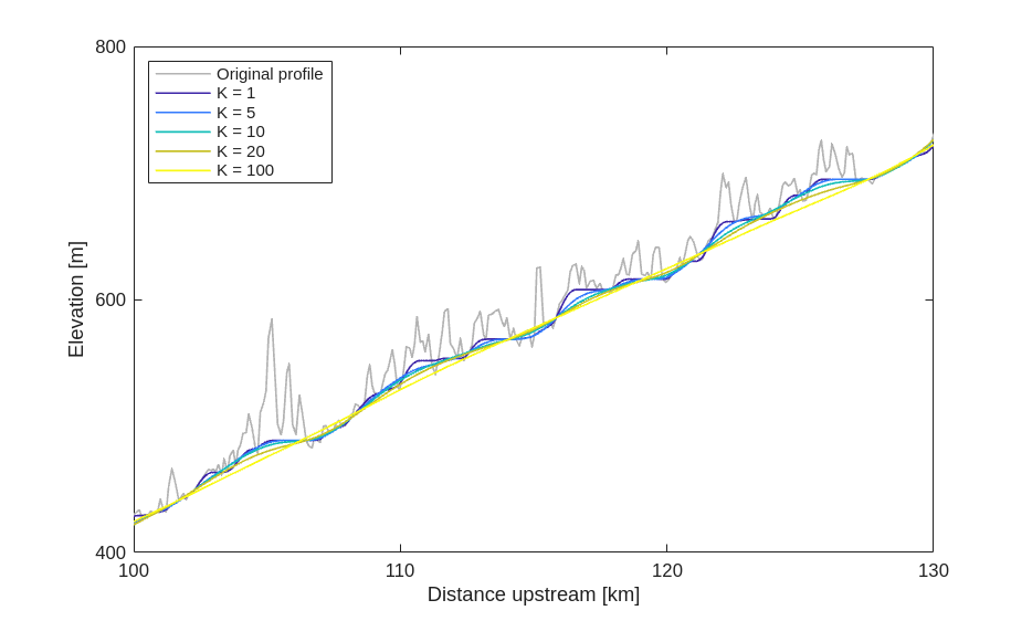
With increasing values of K, stream profiles are getting smoother, while running along a the specified quantile of the profile.

Now which parameters are optimal for your river or river network is to be determined, and I don’t have good recommendations here, except to try out and interpret the results visually. The tool crsapp is helpful here.

Also note that crs (and quantcarve) have additional parameters that let you specify the minimum gradient (so that you can avoid horizontal river sections) or knickpoints, i.e. locations where the profile is allowed to change its gradient abruptly.

References and Additional Information#

Bricker, J.D., Schwanghart, W., Adhikari, B.R., Moriguchi, S., Roeber, V., Giri, S. (2017): Performance of models for flash flood warning and hazard assessment: the 2015 Kali Gandaki landslide breach in Nepal. Mountain Research and Development, 37, 5-15. [DOI: 10.1659/MRD-JOURNAL-D-16-00043.1]