Introduction to TopoToolbox

Welcome to the TopoToolbox Gallery, a collection of user-contributed demonstrations of TopoToolbox!

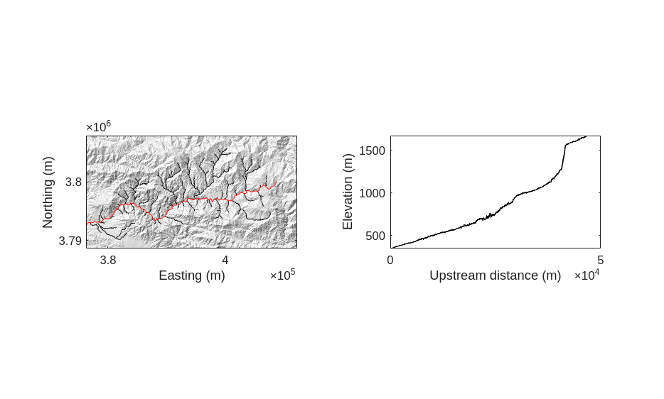
To begin, we will create a hillshade of a digital elevation model of Big Tujunga creek in California. Make sure you have installed TopoToolbox and that it is on your MATLAB path.

The Big Tujunga DEM is provided as one of the example DEMs with TopoToolbox, so we can load it using the GRIDobj constructor.

DEM = GRIDobj('srtm_bigtujunga30m_utm11.tif')

DEM =
  GRIDobj with properties:
           Z: [643x1197 single]
    cellsize: 30
          wf: [2x3 double]
        size: [643 1197]
        name: ''
       zunit: ''
      xyunit: ''
      georef: [1x1 map.rasterref.MapCellsReference]

The DEM is returned as a GRIDobj, TopoToolbox’s representation of single-band raster datasets. To make a hillshade, we can use the imageschs method on the GRIDobj. Instead of using TopoToolbox’s default colormap, we will produce a greyscale hillshade by giving it a single color of white to represent the lightest value. imageschs takes care of shading the DEM.

tiledlayout(1,2)
nexttile
imageschs(DEM,[], colormap=[1, 1, 1], colorbar=false)
xlabel("Easting (m)")
ylabel("Northing (m)")

Now let’s add a visualization of the stream network to this map. We first create a FLOWobj storing flow directions on the DEM and then a STREAMobj that picks out the streams. We also call the klargestconncomps method on this STREAMobj to restrict our analysis to the main watershed.

FD = FLOWobj(DEM);
S  = STREAMobj(FD);
S = klargestconncomps(S, 1);

We can add the STREAMobj to our plot with its plot method.

hold on
plot(S, color='k')
hold off

Finally, let’s use the trunk method on the STREAMobj to pick out the longest stream in the watershed and the plotdz method to plot its profile in another subplot.

T = S.trunk();
hold on
plot(T, color='r')
hold off

ax2 = nexttile;
plotdz(T, DEM, color="black")
xlabel("Upstream distance (m)")
ylabel("Elevation (m)")
ax2.PlotBoxAspectRatio = [1 643/1197 1];