Chi maps of the Rhine-Danube drainage divide (MATLAB)#
Author#
This notebook is licensed under CC-BY 4.0.
Highlighted references#
Winterberg, S., Willett, S.D. Greater Alpine river network evolution, interpretations based on novel drainage analysis. Swiss J Geosci 112, 3–22 (2019). 10.1007/s00015-018-0332-5
Audience#
New users of TopoToolbox interested in tectonic geomorphology.
Introduction#
\(\chi\) maps illustrate the potential for dynamic reorganization of river basins (Willett et al., 2014). They display the value of the \(\chi\) metric (Perron and Royden, 2013) at points along the stream network. \(\chi\) is a quantity that arises when solving the one-dimensional steady-state stream power equation by separation of variables. It is given by the equation
where \(A(x)\) is the drainage area at point \(x\) along the stream network. \(A_0\) is a reference drainage area used to nondimensionalize the integrand. \(m\) and \(n\) are constants. The integration is performed upstream from a location denoted \(x_b\).
Winterberg and Willett compute \(\chi\) for the major rivers draining the Alps and interpret maps of \(\chi\) to understand the transient evolution of these river basins in response to tectonics both within and outside of the Alpine orogen. We will replicate a portion of their \(\chi\) analysis, focusing on the drainage divide between the Rhine and Danube river basins.
To compute \(\chi\), we need to
Load a raster containing elevation data
Compute flow directions
Identify the stream network from these drainage directions
Integrate the inverse of the drainage area upstream
Loading data#
We will load a DEM covering the entire Rhine and Danube drainage basins. We will use the SRTM15+ data (Tozer et al. 2019) from OpenTopography. This is a fairly coarse resolution dataset, but it will show the main features in the $\chi$ map without requiring too much processing time and memory. Try to use a finer dataset like the Copernicus 90 m data and compare the results if you are interested.
[1]:
DEM = readopentopo(west=3, east=30, south=42, north=53, ...
                   demtype='SRTM15Plus');
[1]:
The downloaded DEM is not in a projected coordinate system.
Make sure to project the DEM using GRIDobj/project or
GRIDobj/reproject2utm.
The DEM is a GRIDobj, TopoToolbox’s representation of raster datasets.
The data returned from OpenTopography is in a geographic coordinate system (latitude and longitude). TopoToolbox works best with data in projected coordinate systems, so we will first reproject the data into the ETRS89 coordinate system, which covers continental Europe. The project method on GRIDobj does this for us. We need to supply the coordinate reference system, so we use the EPSG code for the ETRS89 projection. We also give project a resolution to fix the horizontal resolution
to 500 m.
[2]:
DEMr = project(DEM, 3035, 'res', 500.0);
We can visualize this DEM using the GRIDobj.imagesc method. We will use the ttcmap function to generate a nice colormap`.
[3]:
[clr,zlimits] = ttcmap(DEMr,'cmap','france');
imagesc(DEMr)
colormap(clr)
clim(zlimits)
[3]:
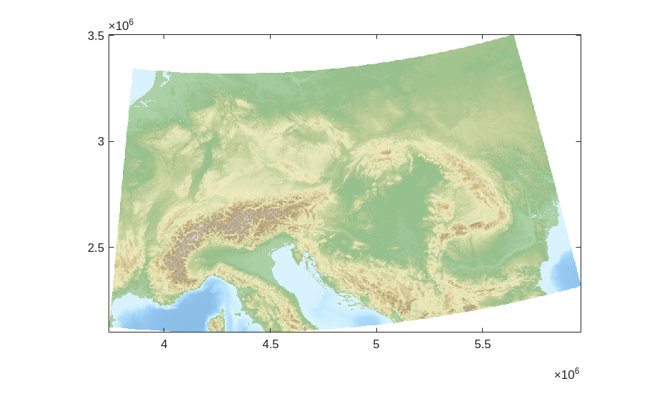
The DEM contains areas below sea level, and one of the assumptions of \(\chi\) analysis is that the stream networks have a common base level at which the upstream integration is started. For simplicity, we will mask out regions with an elevation below 0 m by setting them to NaN, but \(\chi\) analysis can be sensitive to the choice of base level, so it is worth testing your choice of base level.
[4]:
DEMr.Z(DEMr.Z <= 0.0) = NaN;
Identifying the stream network#
Now we are ready to compute the flow directions and the stream network. TopoToolbox represents flow directions using a FLOWobj and stream networks with a STREAMobj. Create the former by giving it the reprojected and masked DEM.
[5]:
FD = FLOWobj(DEMr);
Then create a STREAMobj from the FLOWobj by defining streams as pixels with a minimum drainage area of 10 km^2.
[6]:
S = STREAMobj(FD, 'unit', 'km', 'minarea', 10.0);
This stream network covers the entire DEM, so we restrict it to the Rhine and Danube by using the klargestconncomps method to select the two largest drainage basins. This works because the Rhine and Danube happen to be the two largest basins in the DEM. If you wanted to select different basins (such as the Po and Rhône as in Winterberg and Willett), you would need some more complicated logic here.
[7]:
S = klargestconncomps(S, 2)
[7]:
S =
  STREAMobj with properties:
              size: [2812 4444]
                ix: [454367x1 double]
               ixc: [454367x1 double]
          cellsize: 500
                wf: [2x3 double]
            georef: [1x1 map.rasterref.MapCellsReference]
            IXgrid: [454369x1 double]
                 x: [454369x1 double]
                 y: [454369x1 double]
          distance: [454369x1 double]
    orderednanlist: [501003x1 double]
Computing \(\chi\)#
The \(\chi\) transform integrates the inverse of the upstream area, so we first need to compute the upstream area. The FLOWobj.flowacc method does this.
[8]:
A = flowacc(FD);
And finally, we compute \(\chi\) with the STREAMobj.chitransform method. We give it the drainage area raster and parameters setting the ratio \(m/n=0.45\) and the reference drainage area \(A_0 =1~\mathrm{m^2 }\). These are the parameters given by Winterberg and Willett.
The units of the drainage area raster are in pixels by default. We can correct that by multiplying the drainage area raster by the square of the cellsize, but chitransform will do it for us if we pass correctcellsize=true.
[9]:
c = chitransform(S, A, 'mn', 0.45, 'a0', 1.0,'correctcellsize',true);
The array c contains the \(\chi\) values for every point in our stream network. To visualize the results, we will plot c in a map view colored by \(\chi\) with the Rhine and Danube drainage basins identified.
First, we will identify the two drainage basins. The FLOWobj.drainagebasins method can do this for us, but it will label all of the basins in the DEM, and we would then have to pick out the Rhine and Danube basins from the results. We can do this on our own by picking out the outlets of the Rhine and Danube from our STREAMobj, labeling them with the numbers 1 and 2, and then filling in the rest of the drainage basin with the propagatevaluesupstream function.
[10]:
outlets = streampoi(S,'outlets', 'ix');
db = propagatevaluesupstream(FD, outlets, [1 2], 'fillval', 0);
Plotting the results#
Now we are ready to make our plot. First, we need some colormaps for the drainage basins and \(\chi\) values. These are provided to match the Python version of this notebook
[11]:
dbcmap = [
    1 1 1; % White for other basins
    0.45 0.25 0.00; % Orange for the Rhine
    0.18 0.10 0.40; % Purple for the Danube
    ];

viridis = [
0.26700401  0.00487433  0.32941519
0.26851048  0.00960483  0.33542652
0.26994384  0.01462494  0.34137895
0.27130489  0.01994186  0.34726862
0.27259384  0.02556309  0.35309303
0.27380934  0.03149748  0.35885256
0.27495242  0.03775181  0.36454323
0.27602238  0.04416723  0.37016418
0.2770184   0.05034437  0.37571452
0.27794143  0.05632444  0.38119074
0.27879067  0.06214536  0.38659204
0.2795655   0.06783587  0.39191723
0.28026658  0.07341724  0.39716349
0.28089358  0.07890703  0.40232944
0.28144581  0.0843197   0.40741404
0.28192358  0.08966622  0.41241521
0.28232739  0.09495545  0.41733086
0.28265633  0.10019576  0.42216032
0.28291049  0.10539345  0.42690202
0.28309095  0.11055307  0.43155375
0.28319704  0.11567966  0.43611482
0.28322882  0.12077701  0.44058404
0.28318684  0.12584799  0.44496
0.283072    0.13089477  0.44924127
0.28288389  0.13592005  0.45342734
0.28262297  0.14092556  0.45751726
0.28229037  0.14591233  0.46150995
0.28188676  0.15088147  0.46540474
0.28141228  0.15583425  0.46920128
0.28086773  0.16077132  0.47289909
0.28025468  0.16569272  0.47649762
0.27957399  0.17059884  0.47999675
0.27882618  0.1754902   0.48339654
0.27801236  0.18036684  0.48669702
0.27713437  0.18522836  0.48989831
0.27619376  0.19007447  0.49300074
0.27519116  0.1949054   0.49600488
0.27412802  0.19972086  0.49891131
0.27300596  0.20452049  0.50172076
0.27182812  0.20930306  0.50443413
0.27059473  0.21406899  0.50705243
0.26930756  0.21881782  0.50957678
0.26796846  0.22354911  0.5120084
0.26657984  0.2282621   0.5143487
0.2651445   0.23295593  0.5165993
0.2636632   0.23763078  0.51876163
0.26213801  0.24228619  0.52083736
0.26057103  0.2469217   0.52282822
0.25896451  0.25153685  0.52473609
0.25732244  0.2561304   0.52656332
0.25564519  0.26070284  0.52831152
0.25393498  0.26525384  0.52998273
0.25219404  0.26978306  0.53157905
0.25042462  0.27429024  0.53310261
0.24862899  0.27877509  0.53455561
0.2468114   0.28323662  0.53594093
0.24497208  0.28767547  0.53726018
0.24311324  0.29209154  0.53851561
0.24123708  0.29648471  0.53970946
0.23934575  0.30085494  0.54084398
0.23744138  0.30520222  0.5419214
0.23552606  0.30952657  0.54294396
0.23360277  0.31382773  0.54391424
0.2316735   0.3181058   0.54483444
0.22973926  0.32236127  0.54570633
0.22780192  0.32659432  0.546532
0.2258633   0.33080515  0.54731353
0.22392515  0.334994    0.54805291
0.22198915  0.33916114  0.54875211
0.22005691  0.34330688  0.54941304
0.21812995  0.34743154  0.55003755
0.21620971  0.35153548  0.55062743
0.21429757  0.35561907  0.5511844
0.21239477  0.35968273  0.55171011
0.2105031   0.36372671  0.55220646
0.20862342  0.36775151  0.55267486
0.20675628  0.37175775  0.55311653
0.20490257  0.37574589  0.55353282
0.20306309  0.37971644  0.55392505
0.20123854  0.38366989  0.55429441
0.1994295   0.38760678  0.55464205
0.1976365   0.39152762  0.55496905
0.19585993  0.39543297  0.55527637
0.19410009  0.39932336  0.55556494
0.19235719  0.40319934  0.55583559
0.19063135  0.40706148  0.55608907
0.18892259  0.41091033  0.55632606
0.18723083  0.41474645  0.55654717
0.18555593  0.4185704   0.55675292
0.18389763  0.42238275  0.55694377
0.18225561  0.42618405  0.5571201
0.18062949  0.42997486  0.55728221
0.17901879  0.43375572  0.55743035
0.17742298  0.4375272   0.55756466
0.17584148  0.44128981  0.55768526
0.17427363  0.4450441   0.55779216
0.17271876  0.4487906   0.55788532
0.17117615  0.4525298   0.55796464
0.16964573  0.45626209  0.55803034
0.16812641  0.45998802  0.55808199
0.1666171   0.46370813  0.55811913
0.16511703  0.4674229   0.55814141
0.16362543  0.47113278  0.55814842
0.16214155  0.47483821  0.55813967
0.16066467  0.47853961  0.55811466
0.15919413  0.4822374   0.5580728
0.15772933  0.48593197  0.55801347
0.15626973  0.4896237   0.557936
0.15481488  0.49331293  0.55783967
0.15336445  0.49700003  0.55772371
0.1519182   0.50068529  0.55758733
0.15047605  0.50436904  0.55742968
0.14903918  0.50805136  0.5572505
0.14760731  0.51173263  0.55704861
0.14618026  0.51541316  0.55682271
0.14475863  0.51909319  0.55657181
0.14334327  0.52277292  0.55629491
0.14193527  0.52645254  0.55599097
0.14053599  0.53013219  0.55565893
0.13914708  0.53381201  0.55529773
0.13777048  0.53749213  0.55490625
0.1364085   0.54117264  0.55448339
0.13506561  0.54485335  0.55402906
0.13374299  0.54853458  0.55354108
0.13244401  0.55221637  0.55301828
0.13117249  0.55589872  0.55245948
0.1299327   0.55958162  0.55186354
0.12872938  0.56326503  0.55122927
0.12756771  0.56694891  0.55055551
0.12645338  0.57063316  0.5498411
0.12539383  0.57431754  0.54908564
0.12439474  0.57800205  0.5482874
0.12346281  0.58168661  0.54744498
0.12260562  0.58537105  0.54655722
0.12183122  0.58905521  0.54562298
0.12114807  0.59273889  0.54464114
0.12056501  0.59642187  0.54361058
0.12009154  0.60010387  0.54253043
0.11973756  0.60378459  0.54139999
0.11951163  0.60746388  0.54021751
0.11942341  0.61114146  0.53898192
0.11948255  0.61481702  0.53769219
0.11969858  0.61849025  0.53634733
0.12008079  0.62216081  0.53494633
0.12063824  0.62582833  0.53348834
0.12137972  0.62949242  0.53197275
0.12231244  0.63315277  0.53039808
0.12344358  0.63680899  0.52876343
0.12477953  0.64046069  0.52706792
0.12632581  0.64410744  0.52531069
0.12808703  0.64774881  0.52349092
0.13006688  0.65138436  0.52160791
0.13226797  0.65501363  0.51966086
0.13469183  0.65863619  0.5176488
0.13733921  0.66225157  0.51557101
0.14020991  0.66585927  0.5134268
0.14330291  0.66945881  0.51121549
0.1466164   0.67304968  0.50893644
0.15014782  0.67663139  0.5065889
0.15389405  0.68020343  0.50417217
0.15785146  0.68376525  0.50168574
0.16201598  0.68731632  0.49912906
0.1663832   0.69085611  0.49650163
0.1709484   0.69438405  0.49380294
0.17570671  0.6978996   0.49103252
0.18065314  0.70140222  0.48818938
0.18578266  0.70489133  0.48527326
0.19109018  0.70836635  0.48228395
0.19657063  0.71182668  0.47922108
0.20221902  0.71527175  0.47608431
0.20803045  0.71870095  0.4728733
0.21400015  0.72211371  0.46958774
0.22012381  0.72550945  0.46622638
0.2263969   0.72888753  0.46278934
0.23281498  0.73224735  0.45927675
0.2393739   0.73558828  0.45568838
0.24606968  0.73890972  0.45202405
0.25289851  0.74221104  0.44828355
0.25985676  0.74549162  0.44446673
0.26694127  0.74875084  0.44057284
0.27414922  0.75198807  0.4366009
0.28147681  0.75520266  0.43255207
0.28892102  0.75839399  0.42842626
0.29647899  0.76156142  0.42422341
0.30414796  0.76470433  0.41994346
0.31192534  0.76782207  0.41558638
0.3198086   0.77091403  0.41115215
0.3277958   0.77397953  0.40664011
0.33588539  0.7770179   0.40204917
0.34407411  0.78002855  0.39738103
0.35235985  0.78301086  0.39263579
0.36074053  0.78596419  0.38781353
0.3692142   0.78888793  0.38291438
0.37777892  0.79178146  0.3779385
0.38643282  0.79464415  0.37288606
0.39517408  0.79747541  0.36775726
0.40400101  0.80027461  0.36255223
0.4129135   0.80304099  0.35726893
0.42190813  0.80577412  0.35191009
0.43098317  0.80847343  0.34647607
0.44013691  0.81113836  0.3409673
0.44936763  0.81376835  0.33538426
0.45867362  0.81636288  0.32972749
0.46805314  0.81892143  0.32399761
0.47750446  0.82144351  0.31819529
0.4870258   0.82392862  0.31232133
0.49661536  0.82637633  0.30637661
0.5062713   0.82878621  0.30036211
0.51599182  0.83115784  0.29427888
0.52577622  0.83349064  0.2881265
0.5356211   0.83578452  0.28190832
0.5455244   0.83803918  0.27562602
0.55548397  0.84025437  0.26928147
0.5654976   0.8424299   0.26287683
0.57556297  0.84456561  0.25641457
0.58567772  0.84666139  0.24989748
0.59583934  0.84871722  0.24332878
0.60604528  0.8507331   0.23671214
0.61629283  0.85270912  0.23005179
0.62657923  0.85464543  0.22335258
0.63690157  0.85654226  0.21662012
0.64725685  0.85839991  0.20986086
0.65764197  0.86021878  0.20308229
0.66805369  0.86199932  0.19629307
0.67848868  0.86374211  0.18950326
0.68894351  0.86544779  0.18272455
0.69941463  0.86711711  0.17597055
0.70989842  0.86875092  0.16925712
0.72039115  0.87035015  0.16260273
0.73088902  0.87191584  0.15602894
0.74138803  0.87344918  0.14956101
0.75188414  0.87495143  0.14322828
0.76237342  0.87642392  0.13706449
0.77285183  0.87786808  0.13110864
0.78331535  0.87928545  0.12540538
0.79375994  0.88067763  0.12000532
0.80418159  0.88204632  0.11496505
0.81457634  0.88339329  0.11034678
0.82494028  0.88472036  0.10621724
0.83526959  0.88602943  0.1026459
0.84556056  0.88732243  0.09970219
0.8558096   0.88860134  0.09745186
0.86601325  0.88986815  0.09595277
0.87616824  0.89112487  0.09525046
0.88627146  0.89237353  0.09537439
0.89632002  0.89361614  0.09633538
0.90631121  0.89485467  0.09812496
0.91624212  0.89609127  0.1007168
0.92610579  0.89732977  0.10407067
0.93590444  0.8985704   0.10813094
0.94563626  0.899815    0.11283773
0.95529972  0.90106534  0.11812832
0.96489353  0.90232311  0.12394051
0.97441665  0.90358991  0.13021494
0.98386829  0.90486726  0.13689671
0.99324789  0.90615657  0.1439362];
Our plot is going to focus on the divide between the Rhine and Danube drainage basins. To avoid plotting data outside this region, which can be very slow, we will crop our DEM and drainage basin rasters to the region of interest.
[12]:
bounds = {[4100000 4400000], [2600000 2900000]};
DEMc = resample(crop(DEMr, bounds), 360.0);
dbc = resample(crop(db, bounds), 360.0, 'nearest');
We will also filter the STREAMobj so it only includes points within this bounding box. The STREAMobj.subgraph method takes an array that is 1 for all nodes in the original STREAMobj that you want in the new one. We use the locb output from subgraph to select the corresponding \(\chi\) values.
[13]:
filt = (bounds{1}(1) <= S.x) & (S.x < bounds{1}(2)) & (bounds{2}(1) <= S.y) & (S.y < bounds{2}(2));
[S2, locb] = subgraph(S, filt);
c2 = c(locb);
Now we are ready to make our plot. First, we’ll plot the hillshade of the drainage basins using the imageschs method on the cropped DEM. We give it the cropped drainage basin raster as the second argument and set the colormap as well.
[14]:
imageschs(DEMc,dbc,'colormap',dbcmap,'colorbar',false,'tickstokm',true, exaggerate=10);
alpha 0.75
Now we add the \(\chi\) values with the STREAMobj.plotc method.
[15]:
hold on
plotc(S2,c2, 'xyscale',0.001)
colormap(viridis)
Finally, we will add a colorbar and some nice labels.
[16]:
cc = colorbar;
cc.Label.String = '\chi [m]';
clim([0 40])
xlim([4100 4400])
ylim([2600 2900])
xlabel('East [km]')
ylabel('North [km]')
hold off
[16]:
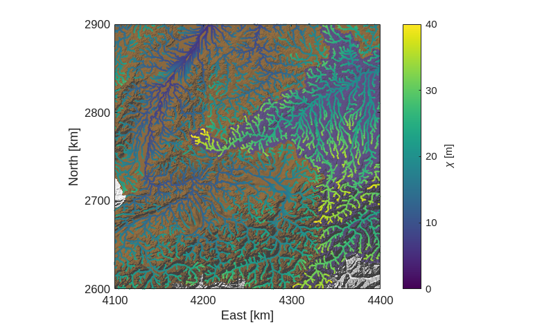
We can easily see from our \(\chi\) map the main feature of the Rhine-Danube divide identified by Winterberg and Willett: the $\chi$ values are much higher in the Danube basin than in the Rhine. The relatively shallower gradients of the Danube are reflected in this asymmetry, which suggests that the drainage divide will migrate into the Danube basin, shrinking it while the Rhine basin grows.
Comparison with Python#
The Python version of this notebook compares the results obtained from TopoToolbox in MATLAB with those obtained from TopoToolbox in Python. To do that, we need to export some data from MATLAB. We’ll identify the trunks of the Rhine and Danube and output their elevation and \(\chi\) values and their drainage basin labels. These will be used to make a \(\chi\) plot in the Python notebook.
[17]:
[ST, loc] = trunk(S);
[STT, loc2] = subgraph(ST, ezgetnal(ST, DEMr) >= 250);
ZTT = ezgetnal(STT, DEMr);
CTT = c(loc);
CTT = CTT(loc2);
DBT  = ezgetnal(STT, db);
writematrix([ZTT CTT DBT],'chiplot.txt');
Additional References#
Tozer, B, Sandwell, D. T., Smith, W. H. F., Olson, C., Beale, J. R., & Wessel, P. (2019). Global bathymetry and topography at 15 arc sec: SRTM15+. Distributed by OpenTopography. https://doi.org/10.5069/G92R3PT9. Accessed 2026-04-21
Perron, J.T. and Royden, L. (2013), An integral approach to bedrock river profile analysis. Earth Surf. Process. Landforms, 38: 570-576. https://doi.org/10.1002/esp.3302