Getting started with TopoToolbox#
This tutorial will guide you through the first steps of getting started with TopoToolbox in Python. For further examples refer to the provided examples.
Installation#
Make sure to have TopoToolbox installed as per the installation guide. If you want to follow along in this notebook, you will also need to download this notebook, install Jupyter Notebook using pip install notebook and launch Jupyter Notebook using jupyter notebook.
Load a DEM and display it#
Before you can actually use the topotoolbox package, it has to be imported. Since we want to plot the DEMs we will also import matplotlib.pyplot.
[1]:
import topotoolbox as tt3
import matplotlib.pyplot as plt
TopoToolbox includes several examples of digital elevation models. To find out which examples are available, use get_dem_names().
[2]:
print(tt3.get_dem_names())
['bigtujunga', 'greenriver', 'kedarnath', 'kunashiri', 'perfectworld', 'taalvolcano', 'taiwan', 'tibet']
Load one of the example files by calling load_dem with the example’s name. TopoToolbox will download the DEM and load it as a GridObject. After the DEM has been created, you can view its attributes by using the info method.
[3]:
dem = tt3.load_dem('bigtujunga')
dem.info()
name: bigtujunga
path: /home/runner/.cache/topotoolbox/bigtujunga.tif
rows: 643
cols: 1197
cellsize: 30.0
bounds: BoundingBox(left=376313.6554542635, bottom=3788627.8276283755, right=412223.6554542635, top=3807917.8276283755)
transform: | 30.00, 0.00, 376313.66|
| 0.00,-30.00, 3807917.83|
| 0.00, 0.00, 1.00|
coordinate system (Projected): EPSG:32611
maximum z-value: 2295.0
minimum z-value: 315.0
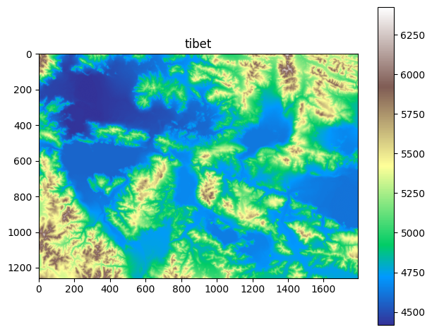
The DEM can be visualized using the plot method on the GridObject.
[4]:
im = dem.plot(cmap="cubehelix")
plt.colorbar(im)
plt.show()
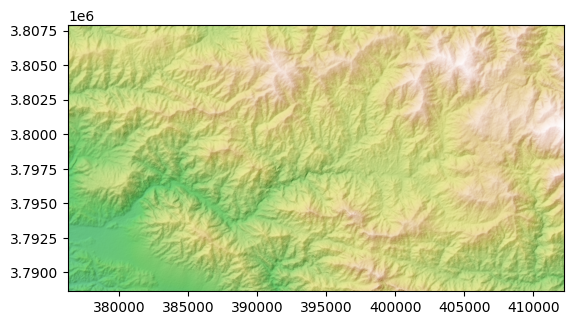
A better impression of the topography can often be gained using hillshading. The GridObject.plot_hs method can be used to plot a hillshade.
[5]:
from matplotlib import colors
import numpy as np

dem.plot_hs(cmap='gist_earth',norm=colors.Normalize(vmin=-1000,vmax=np.nanmax(dem)))
[5]:
<matplotlib.image.AxesImage at 0x7fdc51f409e0>
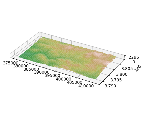
One can also construct a 3D view of the DEM using the GridObject.plot_surface method.
[6]:
fig, ax = plt.subplots(subplot_kw=dict(projection='3d'))
dem.plot_surface(ax=ax, cmap='gist_earth', norm=colors.Normalize(vmin=-1000,vmax=np.nanmax(dem)))
ax.set_aspect('equal')
ax.set_zticks([0,np.nanmax(dem)])
plt.show()
If you have a DEM stored on your computer, you can use the function read_tif to load the data by calling it with the path to the file
tt3.read_tif("/path/to/DEM.tif")
If you have used load_dem to download the example DEMs and would like to remove the examples from your disk, you can use clear_cache to deleted the stored data.
tt3.clear_cache()