Derive, modify and plot the stream network

The stream network is a subset of the flow network. Often, this subset is defined as having a minimum upstream area. The idea is that if upstream area exceeds a critical value than flow becomes channelized in stream networks.

StreamObject stores stream networks. Here we simply assume that streams initiate at upstream areas greater than 1000 pixels.

import topotoolbox as tt3
import matplotlib.pyplot as plt
import numpy as np

dem = tt3.load_dem('bigtujunga')
fd  = tt3.FlowObject(dem)
s   = tt3.StreamObject(fd,threshold=1000,units='pixels')

Plot the stream network

The stream network can be plotted using the plot method on StreamObject.

fig, ax = plt.subplots()
dem.plot(ax,cmap="copper")
s.plot(ax=ax,color='c')
plt.show()

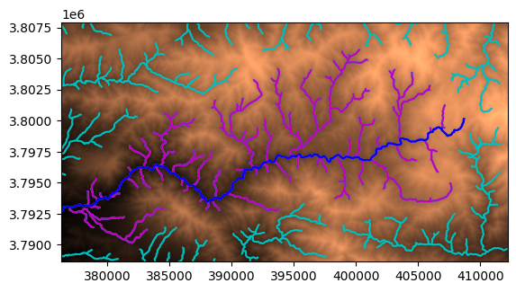
Modify the stream network

Frequently, we might be only interested in parts of the river network. StreamObject has a number of methods that can modify the geometry of the network. For example, we may be interested in only the largest basin.

s2 = s.klargestconncomps(1)
st = s2.trunk()
fig,ax = plt.subplots()
dem.plot(ax=ax,cmap="copper")
s.plot(ax=ax, color='c')
s2.plot(ax=ax,color='m')
st.plot(ax=ax, color='b')
plt.show()

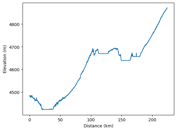
Plot the longitudinal stream profile

Applications in tectonic geomorphology are often interested in longitudinal profiles and features such as knickpoints. Visual inspection of the profile provides a first clue for these features.

fig = plt.figure()
ax = plt.axes(xlabel="Distance (km)", ylabel="Elevation (m)")
st.plotdz(dem, ax=ax, dunit='km')
ax.autoscale_view()

Create a \(\chi\) (chi) map

\(\chi\) maps are a common tool to identify divide migration patterns and assess the relative erosional behaviour of neighboring catchments.

In a \(\chi\) transformation, the distance upstream of a river is replaced by a reference that factors in its total and upstream drainage area and the concavity of the stream:

$:nbsphinx-math:chi `= :nbsphinx-math:int{ frac{A_0}{A(x)^{m/n}}}` dx $

More info in this blogpost: https://topotoolbox.wordpress.com/2017/08/18/chimaps-in-a-few-lines-of-code-final/

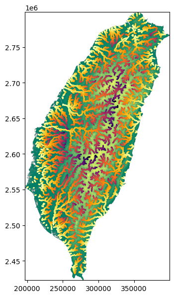
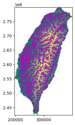
Load a new DEM and extract the stream network

A shared base level is needed for this catchment comparison and we will use the preloaded Taiwan topography.

dem = tt3.load_dem('taiwan')
fd  = tt3.FlowObject(dem)
s   = tt3.StreamObject(fd,threshold=1000,units='pixels')

fig, ax = plt.subplots()
dem.plot(ax,cmap="summer")
s.plot(ax=ax,color='m')
plt.show()

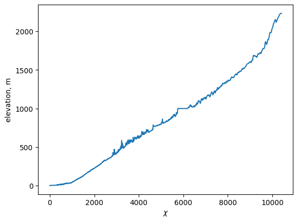
\(\chi\) profile of the longest river

Like the longitudinal long profile above, we can start with a plot of the \(\chi\) profile of the largest river.

For this we will use the chitransform method on a StreamObject. It uses the drainage area information gained from the flow_accumulation method on the FlowObject. The resulting \(\chi\) data is sorted in the same order as the stream elevation from the method ezgetnal. These datapoints are stored in a numpy.array and they do not sequentially traces rivers. We need one extra steps to sort these into tributaries. We will use the StreamObject method xy to achieve and sort the datapoints in sublists of tributaries.

acc = fd.flow_accumulation()     # calculate the flow accumulation (unit=px)

s_chi = s.chitransform(acc)  # chi values for all streams
s_z   = s.ezgetnal(dem)      # elevation values for all streams

s_xy    = s.xy()                    # extract the x, y coordinates of all streams
s_z_chi = s.xy(data=(s_z,s_chi))    # reorganize elevation and chi values in pairs, in the same sublists as the coordinates.

trib_z, trib_chi = zip(*max(s_z_chi, key=len))    # identify the longest river and extract its values.

fig, ax = plt.subplots()
ax.plot(trib_chi,trib_z)
ax.set_xlabel('$\chi$')
ax.set_ylabel('elevation, m')

<>:13: SyntaxWarning: invalid escape sequence '\c'
<>:13: SyntaxWarning: invalid escape sequence '\c'
/tmp/ipykernel_3623/1212303296.py:13: SyntaxWarning: invalid escape sequence '\c'
  ax.set_xlabel('$\chi$')

Text(0, 0.5, 'elevation, m')

Showing \(\chi\) values in map view

To plot the stream network color-coded by its \(\chi\) values, we loop through the sublists created by the method xy on the StreamObject.

fig, ax = plt.subplots(figsize=(14,7))
dem.plot(ax=ax,cmap="summer")

for coord_group, chi_group in zip(s_xy, s_z_chi):   # unpack the sublists one by one to move through the tributaries
    trib_x, trib_y   = zip(*coord_group)                 # extract the coordinates of the tributaries
    trib_z, trib_chi = zip(*chi_group)                   # extract the elevation and chi values of the tributaries

    ax.scatter(trib_x, trib_y, c=trib_chi, cmap='inferno_r', s=0.5, vmin=0, vmax=np.max(s_chi))   # note that we use common min/max values for all tributaries