Metamorphic testing in TopoToolbox 3

Authors

• Will Kearney, University of Potsdam, (homepage, GitHub)

This notebook is licensed under CC-BY 4.0.

Audience

Geoscientific software developers and those interested in the internals of TopoToolbox 3 and its testing framework in particular.

Introduction

A major challenge in testing scientific software is the oracle problem. The simplest approach to software testing assumes that you know the expected output of your program for the inputs you supply – this is the oracle who knows exactly what will happen when you run your program. The test then runs the input through your program and compares its output with the oracle’s output and passes if they are identical or fails if not. If you don’t have an oracle, you have to figure out another way to know when you are correct.

• Test cases with known analytical solutions verify behavior, but they may not accurately capture features of real data.

• Snapshot or characterization tests use the output from previous versions of the software, which verifies that the behavior has not unexpectedly changed, but does not verify that it was correct in the first place.

• Subcomponents may have behavior that can be fully specified and tested, but bugs often arise when integrating subcomponents.

Property-based testing

Another valuable testing method in the absence of oracles is property-based testing. A property-based test specifies properties that should hold of correct output and then verifies these properties on the output of your program. Input data for property-based tests can be randomly generated, because you no longer need to figure out the correct output for any input.

Property-based testing is extensively used in TopoToolbox 3, and one example tests the fillsinks function. When you fill sinks in a DEM using the GridObject.fillsinks method, there shouldn’t be any sinks in the output. Let’s see how that works. First, we’ll import some packages.

import topotoolbox as tt3
import numpy as np
import matplotlib.pyplot as plt

Now we’ll generate a random DEM. Ideally the random DEM would resemble a real world dataset as closely as possible. For this illustration, though, it is just important that we create some sinks, so we’ll just use some Gaussian white noise to generate our data.

rng = np.random.default_rng(0x544f504f)

z = tt3.GridObject()
z.cellsize=1.0
z.z = rng.normal(size=(10,10))
z.plot()

<matplotlib.image.AxesImage at 0x7f3aa8a06d50>

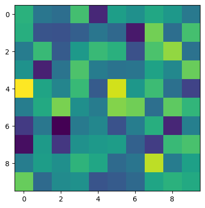
Now that we have a DEM, we need some way to identify sinks in the DEM. A sink is any pixel surrounded by pixels of equal or greater elevation. To be specific, a sink is a pixel where the minimum elevation of its 8 neighbors it is greater than its own elevation. We can compute that minimum elevation using morphological erosion:

def labelsinks(dem):
    return dem.erode(footprint=np.array([[1,1,1],[1,0,1],[1,1,1]])) > dem

Let’s apply that to our random DEM and show the result. Black pixels are sinks and white ones are not sinks.

fig1, (ax1, ax2) = plt.subplots(1, 2)

z.plot(ax=ax1)
labelsinks(z).plot(ax=ax2, cmap="Greys")

<matplotlib.image.AxesImage at 0x7f3aa657a180>

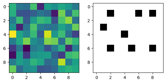
Some of the pixels are black, so there are some sinks in this DEM. This is only the input data, however. We expected there to be sinks, because we want to eliminate them using fillsinks. If there were no sinks in the input data, this test would be useless, because it would not show whether fillsinks actually fills sinks. Let’s create the same plot, but for the DEM that has been run through fillsinks first.

fig2, (ax1, ax2) = plt.subplots(1, 2)

zf = z.fillsinks()

zf.plot(ax=ax1)
labelsinks(zf).plot(ax=ax2, cmap="Greys")

<matplotlib.image.AxesImage at 0x7f3aa643a240>

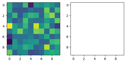
All the pixels are white, which means that this test passes! fillsinks actually does fill the sinks in the DEM.

This property suggests that fillsinks works as expected, but it does not fully specify its behavior. Why not? Think about a way you could implement fillsinks that passes this test but that does not do a good job of filling sinks in the DEM.

If you need a hint: when do you stop filling a sink?

What other properties do you expect a filled DEM to have? Can you write a function that verifies those properties?

Metamorphic testing

Property-based testing is great! You can use real or randomly-generated data to test your functions, and you don’t have to know exactly what the results should look like. Many property-based testing frameworks come with a way to “minimize” a randomly generated test case that creates a small example that fails the test, which makes it easier to debug your code.

The hard part of property-based testing is coming up with the properties and figuring out how to verify them. For the fillsinks test above, we constructed a property by clearly defining a sink and saying that fillsinks should remove all the sinks, and we verified the property using morphological erosion to compute the minimum elevation of a pixel’s neighbors. What if you can’t think of a meaningful property? Or what if you have a property, but you don’t know how to verify it? Can you still use property-based testing?

In some cases, you can, using a technique called metamorphic testing. Instead of specifying and verifying a property that holds over a single invocation of a function like fillsinks, metamorphic testing uses two or more input data sets that are related to each other by a known transformation. If the outputs corresponding to the transformed inputs are also related to each other by a known transformation, then you can verify a property by inverting the transformation on the outputs and making sure they are equal.

This can be a little confusing, so let’s look at an example. GridObject.evansslope computes the magnitude of the gradient for a DEM using a polynomial fit to 3x3 windows. If we rotate the DEM by 90 degrees, the gradient will be oriented differently for each pixel, but it will have the same gradient. Our metamorphic testing relation is

z.evansslope().rotate90() == z.rotate90().evansslope()

TopoToolbox doesn’t have a function that rotates a GridObjects, so let’s implement that. In a real implementation, we should deal with the georeferencing information of GridObjects, but we will ignore that for now and just rotate the data.

def rotGrid90(dem):
    return dem.duplicate_with_new_data(np.rot90(dem))

Now we can run our metamorphic test: rotating then computing gradients should be equal to computing gradients then rotating. Note that we use allclose here rather than array_equal. The rotated DEM will be processed in a different order than the unrotated one, so the non-associativity of floating point arithmetic shows up as very small differences between the results. allclose verifies that the two results are equivalent up to a small tolerance.

np.allclose(rotGrid90(z.evansslope()), rotGrid90(z).evansslope())

True

Sometimes the metamorphic relationship between the outputs is more complicated. GridObject.evansslope can also return the partial derivatives in the x and y directions. These do not pass the rotation test:

np.allclose(rotGrid90(z.evansslope(partial_derivatives=True)[0]), rotGrid90(z.evansslope(partial_derivatives=True)[0]))

True

np.allclose(rotGrid90(z.evansslope(partial_derivatives=True)[1]), rotGrid90(z.evansslope(partial_derivatives=True)[1]))

True

They fail because the x and y axes switch positions during the rotation. If we instead compare the x derivative to the negated y derivative, the test does pass:

np.allclose(rotGrid90(z.evansslope(partial_derivatives=True)[0]), rotGrid90(z.evansslope(partial_derivatives=True)[1]))

False

np.allclose(rotGrid90(z.evansslope(partial_derivatives=True)[1]), rotGrid90(z.evansslope(partial_derivatives=True)[0]))

False

Metamorphic testing can be easier than other forms of property-based testing, but it does require some careful thought about how the transformation affects the output data.

Metamorphic testing of memory ordering in TopoToolbox

Metamorphic testing has been very useful in ensuring that TopoToolbox 3 is able to operate on GridObjects regardless of their underlying memory order.

A GridObject represents a two-dimensional raster dataset. These data are stored in memory as a one-dimensional array in one of two memory layouts. The row-major layout places the elements of a single row next to each other in order of increasing column index. All of the elements of one row are stored before the elements of the next row. The column-major layout places the elements of a single column next to each other in order of increasing row index. Numpy arrays are row-major by default but can also be column-major. MATLAB arrays are column-major.

libtopotoolbox, the C library powering both pytopotoolbox and the MATLAB package, can handle arrays in either order, but it requires the caller of a function that uses two-dimensional arrays to supply the dimensions of that array with the dimension whose index increases fastest first. For column-major arrays, this is the row dimension, so libtopotoolbox functions are called with dims={rows, columns}. For row-major arrays, libtopotoolbox functions are called with dims={columns, rows}. This ensures that libtopotoolbox iterates over the dimension whose elements are laid out next to each other in memory first, which is usually the fastest way to access data in modern CPUs.

This works well for many functions like fillsinks, but metamorphic testing discovered a bug in how libtopotoolbox handles memory ordering during flow routing. This bug was fixed in pull request #186. Here, we will illustrate how this bug was detected using metamorphic testing.

We start by generating a random DEM as above.

cdem = tt3.GridObject()
cdem.cellsize=1.0
cdem.z = rng.normal(size=(21,23))

Numpy arrays are row-major by default, which can be confirmed by checking the flags attribute of the Numpy array inside the GridObject.

cdem.z.flags

  C_CONTIGUOUS : True
  F_CONTIGUOUS : False
  OWNDATA : True
  WRITEABLE : True
  ALIGNED : True
  WRITEBACKIFCOPY : False

The C_CONTIGUOUS flag indicates that it is stored in row-major order. If F_CONTIGUOUS were true, it would be stored in column major order.

Next, we copy the data into a new GridObject, but we change the storage order. Verify that it is column-major by checking the flags.

fdem = cdem.duplicate_with_new_data(np.array(cdem, order='F'))
fdem.z.flags

  C_CONTIGUOUS : False
  F_CONTIGUOUS : True
  OWNDATA : True
  WRITEABLE : True
  ALIGNED : True
  WRITEBACKIFCOPY : False

When operating on arrays, Numpy implicitly converts to the same memory order, so these two GridObjects compare equal despite not being laid out identically in memory. We will use this property to verify the results of flow routing later.

np.array_equal(cdem, fdem)

True

TopoToolbox automatically handles swapping the dimensions to the order that libtopotoolbox expects with the dims attribute on GridObjects. The shape attribute returns the rows and columns, in that order, regardless of the memory layout.

fdem.shape

(21, 23)

cdem.shape

(21, 23)

But the dims attribute reverses these for row-major arrays.

fdem.dims

(21, 23)

cdem.dims

(23, 21)

Now we will route flow. PR #186 fixed the default behavior of flow routing, so to replicate it, we will need our own flow routing function. This does basically the same thing as the FlowObject constructor, but it takes an additional order parameter that we will use to control how libtopotoolbox handles the memory ordering. A value of 0 represents column-major ordering and 1 represents row-major ordering. For now, though, we will ignore this argument.

We don’t package the resulting list of edges in the flow network into a FlowObject for simplicity.

def flow_routing_d8(dem, order):
    (aux, filled_dem, flats) = dem.auxiliary_topography(None, True)

    node = np.zeros_like(aux, dtype=np.int64)
    direction = np.zeros_like(aux, dtype=np.uint8)
    tt3._grid.flow_routing_d8_carve(node, direction, filled_dem, aux, flats, dem.dims, 0)

    source = np.zeros(aux.size, dtype=np.int64)
    target = np.zeros(aux.size, dtype=np.int64)
    edge_count = tt3._grid.flow_routing_d8_edgelist(source, target, node, direction, dem.dims, 0)

    return (direction, source[0:edge_count], target[0:edge_count])

cdirection, csource, ctarget = flow_routing_d8(cdem, 1)
fdirection, fsource, ftarget = flow_routing_d8(fdem, 0)

We can compare these lists of edges:

np.array_equal(csource, fsource)

False

np.array_equal(ctarget, ftarget)

False

To find that they are not identical. Unfortunately, this doesn’t work even if the flow routing behaves correctly. The values of the source and target arrays are linear indices into the two-dimensional array, and they change depending on whether your array is in row-major or column-major. It is also not possible to convert the row-major indices into column-major indices and compare because the topological ordering in which the arrays are stored is not unique. It can vary depending on the order in which pixels are visited in each array, which, again, is different for row- and column-major arrays.

We need a better way to compare the flow networks. In the pytopotoolbox test suite, we compare them by putting the edges into a set data structure and computing the set difference. This is insensitive to the topological ordering, but it is not particularly easy to visualize. Instead, we will compute the flow accumulation and compare that for the two memory orderings. Because we don’t have FlowObjects, we have to write our own flow accumulation function. We will do this purely in Python instead of using libtopotoolbox.

def flow_accumulation(source, target, size, order):
    a = np.ones(size, order='F' if order == 0 else 'C')

    for (u, v) in zip(source, target):
        ui = np.unravel_index(u, size, order='F' if order == 0 else 'C')
        vi = np.unravel_index(v, size, order='F' if order == 0 else 'C')
        a[vi] = a[vi] + a[ui]

    return a

ca = flow_accumulation(csource, ctarget, cdem.shape, 1)
fa = flow_accumulation(fsource, ftarget, fdem.shape, 0)
np.array_equal(ca, fa)

False

Our metamorphic test has failed: different memory layouts produce different answers. How does this happen? Let’s zoom in on one of the patches where the test failed and look at the elevation values around that patch.

cux, cuy = np.unravel_index(csource, cdem.shape, order='C')
cvx, cvy = np.unravel_index(ctarget, cdem.shape, order='C')

fux, fuy = np.unravel_index(fsource, cdem.shape, order='F')
fvx, fvy = np.unravel_index(ftarget, cdem.shape, order='F')

idxs = np.arange(0, np.prod(cdem.shape)).reshape(cdem.shape)
cidxs = np.zeros(cdem.shape, dtype=np.int64)
cidxs[cux, cuy] = idxs[cvx, cvy]
fidxs = np.zeros(cdem.shape, dtype=np.int64)
fidxs[fux, fuy] = idxs[fvx, fvy]

i = fux[fidxs[fux, fuy] != cidxs[fux, fuy]][10]
j = fuy[fidxs[fux, fuy] != cidxs[fux, fuy]][10]

It helps to look at the filled DEM rather than the original. fillsinks does not depend on the memory layout, so we only need to do this once. Implement the metamorphic test for fillsinks if you are not convinced.

filled_dem = cdem.fillsinks()
filled_dem[i-1:i+2, j-1:j+2]

array([[ 0.701136  , -0.24139445,  1.5674267 ],
       [ 0.25242442,  1.3833117 , -0.6821779 ],
       [ 1.0147583 , -0.6821779 , -0.2839691 ]], dtype=float32)

The center pixel is surrounded by pixels with the same elevation to the left, bottom and right. The maximum gradient is to the cardinal neighbors to the left, bottom and right of the center pixel. The gradient to the diagonal neighbors with the same elevation is shallower because it is scaled by the square root of two.

The bug arises when neighbors have the same downward gradient. flow_routing_d8_carve chooses the bottom neighbor for the row-major DEM but the right neighbor for the column-major DEM.

D8 flow routing checks the downward gradient of each of the eight neighbors consecutively and chooses the neighbor with the largest downward gradient. If two neighbors have the same downward gradient, the first neighbor encountered is chosen. Prior to pull request #186, the scan was conducted in two different directions for row- and column-major arrays. Neighborhoods were scanned in the counterclockwise direction starting from the bottom for row-major arrays and in the opposite direction starting from the east for column-major arrays.

To fix this, the order parameter was added to libtopotoolbox flow routing functions. This parameter switches the direction of the neighborhood scan for row-major arrays. Let’s now pass our order parameter to the flow routing functions and compare the flow accumulations again.

def flow_routing_d8_correct(dem, order):
    (aux, filled_dem, flats) = dem.auxiliary_topography(None, True)

    node = np.zeros_like(aux, dtype=np.int64)
    direction = np.zeros_like(aux, dtype=np.uint8)
    tt3._grid.flow_routing_d8_carve(node, direction, filled_dem, aux, flats, dem.dims, order)

    source = np.zeros(aux.size, dtype=np.int64)
    target = np.zeros(aux.size, dtype=np.int64)
    edge_count = tt3._grid.flow_routing_d8_edgelist(source, target, node, direction, dem.dims, order)

    return (source[0:edge_count], target[0:edge_count])

csource2, ctarget2 = flow_routing_d8_correct(cdem, 1)
fsource2, ftarget2 = flow_routing_d8_correct(fdem, 0)

ca2 = flow_accumulation(csource2, ctarget2, cdem.shape, 1)
fa2 = flow_accumulation(fsource2, ftarget2, fdem.shape, 0)

np.array_equal(ca2, fa2)

True

The flow accumulations are now equal and the metamorphic test passes.

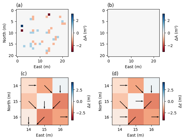
Finally, let’s visualize the flow accumulation differences and the pixel neighborhoods we just examined.

fig5 = plt.figure(layout="constrained")
spec = fig5.add_gridspec(2, 2)

vm1 = np.max(np.abs(filled_dem[i-1:i+2, j-1:j+2] - filled_dem[i,j]))

ax2 = fig5.add_subplot(spec[1, 0])

pm2 = ax2.imshow(filled_dem - filled_dem[i,j], vmin=-2*vm1, vmax=2*vm1, cmap="RdBu")
ax2.quiver(cuy, cux, (cvy - cuy), (cvx - cux), angles='xy', color='k', zorder=2, scale=6, width=0.01)
ax2.set_ylim(i+1.5, i-1.5)
ax2.set_xlim(j-1.5, j+1.5)
ax2.set_yticks([i-1, i, i+1])
ax2.set_xticks([j-1, j, j+1])
ax2.set_title("(c)", loc="left")
ax2.set_xlabel("East (m)")
ax2.set_ylabel("North (m)")


ax5 = fig5.add_subplot(spec[1, 1])

ax5.imshow(filled_dem - filled_dem[i,j], vmin=-2*vm1, vmax=2*vm1, cmap="RdBu")
ax5.quiver(fuy, fux, (fvy - fuy), (fvx - fux), angles='xy', color='k', zorder=2, scale=6, width=0.01)
ax5.set_ylim(i+1.5, i-1.5)
ax5.set_xlim(j-1.5, j+1.5)
ax5.set_yticks([i-1, i, i+1])
ax5.set_xticks([j-1, j, j+1]);
ax5.set_title("(d)", loc="left")
ax5.set_xlabel("East (m)")
ax5.set_ylabel("North (m)")



fig5.colorbar(pm2, ax=[ax2], shrink=0.8, label="Δz (m)")
fig5.colorbar(pm2, ax=[ax5], shrink=0.8, label="Δz (m)")


ax3 = fig5.add_subplot(spec[0, 0])

pm = ax3.imshow(ca - fa, cmap="RdBu", vmin=-3, vmax=3)
ax3.set_title("(a)", loc="left")
ax3.set_xlabel("East (m)")
ax3.set_ylabel("North (m)")


ax6 = fig5.add_subplot(spec[0, 1])
ax6.imshow(ca2 - fa2, cmap="RdBu", vmin=-3, vmax=3)
ax6.set_title("(b)", loc="left")
ax6.set_xlabel("East (m)")

fig5.colorbar(pm, ax=[ax3], shrink=0.8, label=r"ΔA (m²)")
fig5.colorbar(pm, ax=[ax6], shrink=0.8, label=r"ΔA (m²)")

<matplotlib.colorbar.Colorbar at 0x7f3aa63e8da0>

References

An overview of how property-based testing is used in real-world software engineering is available in

• Harrison Goldstein, Joseph W. Cutler, Daniel Dickstein, Benjamin C. Pierce, and Andrew Head. 2024. Property-Based Testing in Practice. In Proceedings of the IEEE/ACM 46th International Conference on Software Engineering (ICSE ‘24). Association for Computing Machinery, New York, NY, USA, Article 187, 1–13. https://doi.org/10.1145/3597503.3639581

A good survey of metamorphic testing is provided by

• Tsong Yueh Chen, Fei-Ching Kuo, Huai Liu, Pak-Lok Poon, Dave Towey, T. H. Tse, and Zhi Quan Zhou. 2018. Metamorphic Testing: A Review of Challenges and Opportunities. ACM Comput. Surv. 51, 1, Article 4 (January 2019), 27 pages. https://doi.org/10.1145/3143561