Using Landlab with TopoToolbox

Author

• Will Kearney, University of Potsdam, (homepage, GitHub)

This notebook is licensed under CC-BY 4.0.

Highlighted references

This notebook implements a variant of the landscape evolution model in

Andy Wickert and Nicole Gasparini. Modeling Hillslopes and Channels with Landlab.. Accessed 22-04-2026.

See there for more details on the model and additional references.

Audience

• Users of TopoToolbox interested in Landlab

• Users of Landlab who would like to use TopoToolbox

Introduction

Landlab is an open source modeling framework for Earth surface dynamics.

With the introduction of the Python interface to TopoToolbox, you can now use TopoToolbox alongside Landlab.

This notebook shows off this capability in two steps. First, we set up a landscape evolution model in Landlab and then use TopoToolbox to analyze and visualize its output. Then we replace one of the components of the model with a TopoToolbox function.

To get started, let’s import some libraries including Landlab and TopoToolbox.

from landlab import RasterModelGrid
from landlab.components import LinearDiffuser, StreamPowerEroder, FlowAccumulator, FlowDirectorD8
from landlab import Component

import topotoolbox as tt3

import matplotlib.pyplot as plt
import numpy as np

from rasterio import Affine
from rasterio.coords import BoundingBox

Using Landlab grids in TopoToolbox

Landlab and TopoToolbox each have their own way of representing gridded datasets. Landlab has a variety of grid types that inherit from the ModelGrid class, and data are contained in fields attached to different elements of grid. TopoToolbox provides the GridObject class, which is a single dataset on a raster grid with equal spacing in the horizontal directions. TopoToolbox GridObjects are roughly equivalent to a single node-based field on a RasterModelGrid, and it is straightforward to convert from a RasterModelGrid field to a GridObject. The following function extracts a node-based field by name from a RasterModelGrid and returns a GridObject.

def from_RasterModelGrid(grid, field):
    """
    Convert a RasterModelGrid into a GridObject

    Returns
    -------
    GridObject

    Raises
    ------
    ValueError
       If the supplied grid does not have equal horizontal spacing.
    """
    # Create an empty GridObject
    dem = tt3.GridObject()

    if grid.dx != grid.dy:
        raise ValueError("Grid must have equal x and y spacing")

    # Set the cellsize
    dem.cellsize = grid.dx

    # Extract the field from the grid and reshape it into a 2D array.
    dem.z = np.array(grid.at_node[field].reshape(grid.shape))

    # Landlab grids typically don't have external
    # coordinate reference systems, but TopoToolbox
    # needs these to plot correctly.
    dem.transform = Affine(grid.dx, 0, 0, 0, -grid.dx, grid.dx * grid.shape[0])
    dem.bounds = BoundingBox(
        top=grid.dx * grid.shape[0],
        bottom=0,
        left=0,
        right=grid.dx * grid.shape[1]
    )

    return dem

Now we can set up and run the model. This is quite similar to the original Landlab example, and we won’t discuss the model in great detail here.

First we create the Landlab grid.

nx = 150
dxy = 50.0
mg = RasterModelGrid((nx, nx), dxy)

Initialize the elevations to small random values.

np.random.seed(0)

mg_noise = np.random.rand(mg.number_of_nodes)
zr = mg.add_field("topographic__elevation", mg_noise)

Set up some parameters in the model.

uplift_rate = 0.001
K_sp = 1.0e-5
m_sp = 0.5
n_sp = 1.0
K_hs = 0.05

And use those parameters to initialize the process components.

frr = FlowAccumulator(mg)
spr = StreamPowerEroder(mg, K_sp=K_sp, m_sp=m_sp, n_sp=n_sp, threshold_sp=0.0)
dfn = LinearDiffuser(mg, linear_diffusivity=K_hs, deposit=False)

Set up the time frame for the model run.

dt = 1000
total_time = 0
tmax = 1e6

t = np.arange(0, tmax, dt)

And run the model!

for ti in t:
    zr[mg.core_nodes] += uplift_rate * dt

    # Diffuse
    dfn.run_one_step(dt)

    # Route flow
    frr.run_one_step()

    # Incise
    spr.run_one_step(dt)
    total_time += dt

Now we will use TopoToolbox to visualize the stream network generated by the model. We convert the topographic__elevation field to a GridObject using our helper function from earlier.

dem = from_RasterModelGrid(mg, "topographic__elevation")

Then we use TopoToolbox’s flow routing to determine the flow directions and identify the stream network from a drainage area threshold. The flow directions are stored in a FlowObject, and the stream network in a StreamObject.

fd = tt3.FlowObject(dem)
s = tt3.StreamObject(fd, units='pixels', threshold=25)

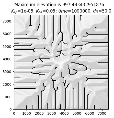
Finally, we make a hillshade of the simulated DEM using the GridObject.plot_hs method and plot the StreamObject on top of it.

from matplotlib.colors import ListedColormap

fig, ax = plt.subplots()

dem.plot_hs(ax=ax, cmap=ListedColormap([0.9, 0.9, 0.9]),
            exaggerate=3)
s.plot(ax=ax, color='k')

plt.title(
    f"$K_{{sp}}$={K_sp}; $K_{{hs}}$={K_hs}; $time$={total_time}; $dx$={dxy}")

max_elev = np.max(zr)
suptitle_text = "Maximum elevation is " + str(max_elev)
plt.suptitle(suptitle_text)

plt.show()

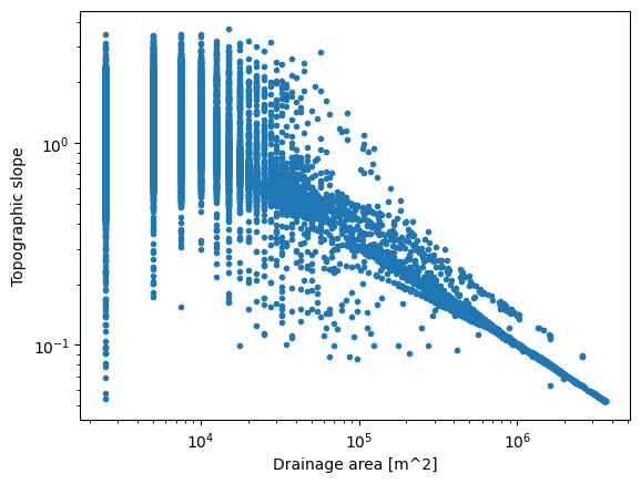
We can also reconstruct the slope-area relationship plotted in the Landlab example. We’ll first need to remove the edges on the boundary from the FlowObject. TopoToolbox tries to route flow along the boundary where possible, but in the Landlab model the boundary nodes are fixed. They will show up as outliers on our plot. We can, however, remove the edges in the FlowObject along the boundary with the following function.

def mask_edges(fd):
    mask = np.ones(fd.shape, dtype=bool)
    mask[1:-1,1:-1] = False
    interior_edges = ~mask[fd.source_indices]
    fd.source = fd.source[interior_edges]
    fd.target = fd.target[interior_edges]
    return fd

fd = mask_edges(fd)

a = fd.flow_accumulation() * dem.cellsize**2
g = dem.gradient8()

indices = np.unravel_index(fd.source, fd.shape)

plt.loglog(a.z[indices], g.z[indices], ".")

plt.xlabel("Drainage area [m^2]")
plt.ylabel("Topographic slope")

Text(0, 0.5, 'Topographic slope')

Using TopoToolbox within a Landlab model

The previous example showed how to use TopoToolbox to visualize the output of a Landlab model run. This is made easier with pytopotoolbox, but you could do the same thing using TopoToolbox in MATLAB by saving the model results and importing them in MATLAB.

Using TopoToolbox to analyze data during a Landlab model run or to implement the process models is a new power unlocked by pytopotoolbox. We will now modify the model run above to do both.

As we have seen above, Landlab does not usually control the time stepping/event loop of your model. Instead, one repeatedly calls a single run_one_step function on different components to update the model grid’s fields of data. Each of these components has a set of input fields and output fields that it requires.

Objects like FlowAccumulator are classes that inherit from Landlab’s base Component class. One does not necessarily need to implement a Component to operate within a Landlab model. You could write a function:

def perform_update(grid):
    # ... Update the arrays of data in `grid`.

and call that every time step. Indeed this is more or less how run_one_step works. The Component class is there more for documentation purposes and to hide implementation details.

We will nonetheless write a component for flow routing using TopoToolbox. This will replace the FlowAccumulator component used above.

Here is the component definition in its entirety.

class TT3FlowRouter(Component):
    """Route flow using TopoToolbox

    Parameters
    ----------

    grid: RasterModelGrid
        Landlab RasterModelGrid object
    """

    _name = "TT3FlowRouter"
    _unit_agnostic = False

    _info = {
        "topographic__elevation": {
            "dtype": float,
            "intent": "in",
            "optional": False,
            "units": "m",
            "mapping": "node",
            "doc": "Land surface topographic elevation",
        },
        "drainage_area": {
            "dtype": float,
            "intent": "out",
            "optional": False,
            "units": "m**2",
            "mapping": "node",
            "doc": "Upstream accumulated surface area contributing to the node's discharge",
        },
        "flow__upstream_node_order": {
            "dtype": int,
            "intent": "out",
            "optional": False,
            "units": "-",
            "mapping": "node",
            "doc": "Node array containing downstream-to-upstream ordered list of node IDs",
        },
        "flow__link_to_receiver_node": {
            "dtype": int,
            "intent": "out",
            "optional": False,
            "units": "-",
            "mapping": "node",
            "doc": "ID of link downstream of each node, which carries the discharge",
        },
        "flow__receiver_node": {
            "dtype": int,
            "intent": "out",
            "optional": False,
            "units": "-",
            "mapping": "node",
            "doc": "Node array of receivers (node that receives flow from current node)",
        },
    }

    def __init__(self, grid):
        super().__init__(grid)

        self._grid = grid

        self._elevation = grid.at_node["topographic__elevation"]

        self.dem = from_RasterModelGrid(self._grid, "topographic__elevation")

        self.fd = tt3.FlowObject(self.dem)

        self.initialize_output_fields()

        self._node = grid.at_node["flow__upstream_node_order"]
        self._receivers = grid.at_node["flow__receiver_node"]
        self._links = grid.at_node["flow__link_to_receiver_node"]
        self._drainage_area = grid.at_node["drainage_area"]

    def set_node(self, fd):
        # Set the "flow__upstream_node_order" field. This is a
        # topologically sorted list of nodes, which is available in
        # the `stream` member of the FlowObject.
        self._node[:] = np.flip(fd.stream.flatten())

    def set_receivers(self, fd):
        # Set the "flow__receiver_node" field. This is the target of each
        # source or the node's own index if it is not a source of any
        # edge. This is straightforward to do with the source and
        # target lists in the FlowObject
        self._receivers[:] = np.arange(len(self._receivers))
        self._receivers[fd.source] = fd.target

    def set_links(self, fd):
        # Set the "flow__link_to_receiver_node" field. This is the
        # most complicated one. This is the link representing the edge
        # in our edge list. Landlab labels links in the Grid regardless
        # whether they carry flow or not, but a FlowObject only records
        # links that carry flow. To get the Landlab link IDs, we need
        # to go through a rather complicated process of checking which
        # link matches the target node for each source. There may be a
        # better way to do this.

        # For every node that does not have a downstream neighbor, the
        # field is set to -1.
        self._links[:] = -1

        # First, find the link IDs of the 8 neighbors of each source
        # node. This is an Nedges x 8 array containing the link IDs of
        # each edge adjacent to each source node or -1 if that edge
        # does not exist.
        links = self._grid.d8s_at_node[fd.source]

        # This is an Nedges x 8 x 2 array representing the two
        # endpoints of each edge. Because of the -1s in the links,
        # this includes some erroneous edges. We will filter those out
        # later.
        endpoints = self._grid.nodes_at_d8[links]

        # Now we check to see if either of the two endpoints is equal
        # to the target. We need to do some reshaping to get numpy to
        # broadcast this correctly.
        mask = np.any(endpoints == np.expand_dims(
            np.stack((fd.target, fd.target), 1), 1), axis=2)

        # Finally, we filter out the erroneous edges by ensuring that
        # the corresponding entry in the links array is not
        # -1. Indexing the links array by this mask gives us the link
        # ID for each edge, which we assign to the source pixels in
        # the "flow__link_to_receiver_node" field.
        self._links[fd.source] = links[np.logical_and(mask, links != -1)]

    def set_drainage_area(self, fd):
        # Lastly, we need the drainage area, which we compute with the
        # flow accumulation. There is a bit of a problem of data types
        # here: we expect float32, Landlab provides float64, so we
        # allocate a new array and copy. pytopotoolbox will eventually support
        # flow network traversals with float64 data.
        interior = np.zeros(fd.shape)
        interior[1:-1,1:-1] = 1.0
        a = np.array(fd.flow_accumulation(weights=interior), dtype=np.float64)

        self._drainage_area[:] = fd.cellsize**2 * a.flatten()

    # This is where we actually do the flow routing.
    def run_one_step(self):
        """
        Compute flow network and flow accumulation
        """
        # Since the elevation may change from time step to time step,
        # we need to construct the GridObject every time.
        self.dem = from_RasterModelGrid(self._grid, "topographic__elevation")

        # Route flow with the FlowObject.
        self.fd = tt3.FlowObject(self.dem)

        # Remove edges that are on the boundary of the DEM.
        mask_edges(self.fd)

        # Now we need to fill in our output fields for Landlab.  These
        # are the important fields that the StreamPowerEroder
        # uses.
        self.set_node(self.fd)
        self.set_receivers(self.fd)
        self.set_links(self.fd)
        self.set_drainage_area(self.fd)

Now that we have our component, we can replicate the diffusion/stream power model above, but using TT3FlowRouter instead of FlowAccumulator. To be able to compare results at the end, we will run the model twice, once with the FlowAccumulator and once with the TT3FlowRouter.

# Set up the grid
nx = 150
dxy = 50.0
mg_tt = RasterModelGrid((nx, nx), dxy)
mg_ll = RasterModelGrid((nx, nx), dxy)

np.random.seed(0x425e5feb)

mg_noise = np.random.rand(mg_tt.number_of_nodes)
zr_tt = mg_tt.add_field("topographic__elevation", np.array(mg_noise, copy=True))
zr_ll = mg_ll.add_field("topographic__elevation", np.array(mg_noise, copy=True))

The main difference between the Landlab and TopoToolbox components is how they route flow through depressions and flat areas. These exist primarily at the beginning of the simulation before the random initial conditions have been smoothed out from diffusion and erosion. To minimize the impact of these differences, we will use TopoToolbox’s imposemin function to carve a channel with a minimum downward slope through the initial conditions. If you would like to see how the two simulations look without the minimum imposition, skip the next cell.

z1 = from_RasterModelGrid(mg_tt, "topographic__elevation")
f1 = tt3.FlowObject(z1)
zz = tt3.imposemin(f1, z1, minimum_slope=1e-5)
zr_tt[:] = zz.z.flatten()
zr_ll[:] = zz.z.flatten()

K_sp = 1.0e-5
m_sp = 0.5
n_sp = 1.0
K_hs = 0.05

Now we set up the components as before. We’ll use the TT3FlowRouter in the first simulation and the FlowAccumulator in the second. TopoToolbox currently always routes flow through depressions, so for better comparison with TopoToolbox, we turn on the DepressionFinderAndRouter in the Landlab FlowAccumulator.

frr_tt = TT3FlowRouter(mg_tt)
spr_tt = StreamPowerEroder(mg_tt, K_sp=K_sp, m_sp=m_sp, n_sp=n_sp, threshold_sp=0.0)
dfn_tt = LinearDiffuser(mg_tt, linear_diffusivity=K_hs, deposit=False)

frr_ll = FlowAccumulator(mg_ll, flow_director=FlowDirectorD8, depression_finder="DepressionFinderAndRouter")
spr_ll = StreamPowerEroder(mg_ll, K_sp=K_sp, m_sp=m_sp, n_sp=n_sp, threshold_sp=0.0)
dfn_ll = LinearDiffuser(mg_ll, linear_diffusivity=K_hs, deposit=False)

dt = 1000
total_time = 0e6
tmax = 2.5e6

t = np.arange(total_time, tmax, dt)

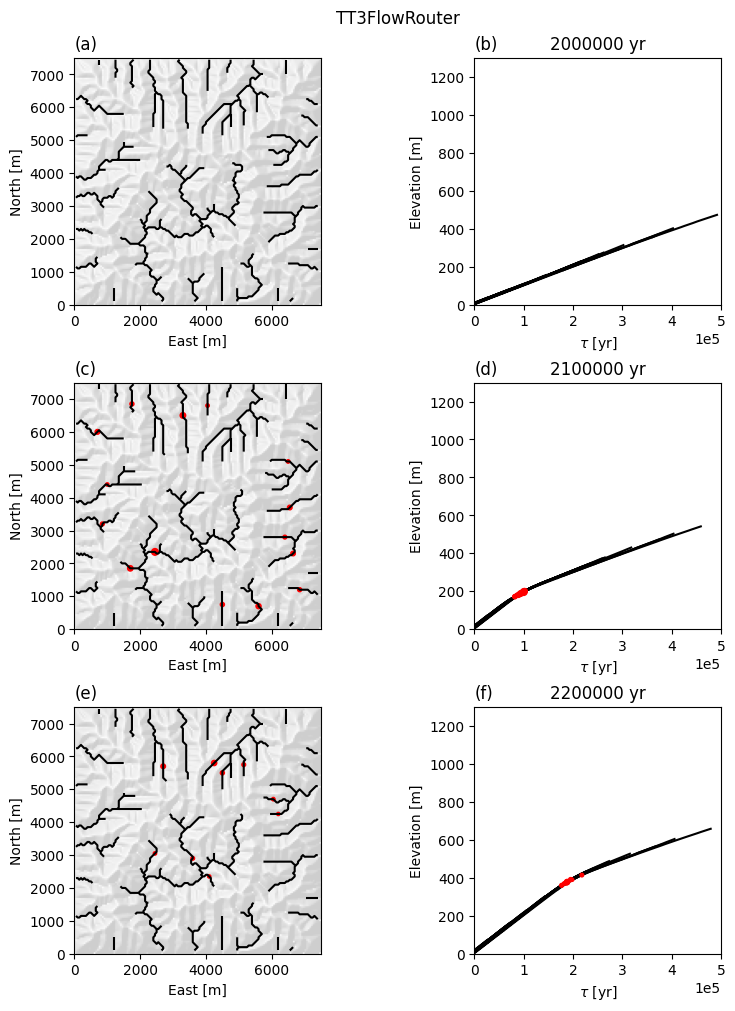
In addition to using the TT3FlowRouter, we will also generate and track knickpoints using TopoToolbox’s knickpointfinder. To make knickpoints, we’ll double the uplift rate after 2 million years of simulation time.

def uplift(t):
    if t < 2e6:
        return 0.001
    if 2e6 <= t < 3e6:
        return 0.002

This is the plotting function that we will use to create plots during the model run. It identifies knickpoints using the knickpoint finder and then plots the stream network and the stream profile in \(\chi\) space.

def plot_knicks(dem, fd, ti, ax1, ax2, labels):
    s = tt3.StreamObject(fd, units='pixels', threshold=100)

    # Mask out the boundary pixels (cf. the mask_edges function above)
    mask = np.zeros((nx,nx), dtype=bool)
    mask[1:-1,1:-1] = True
    mask[2:-2,2:-2] = False
    s = s.upstreamto(s.ezgetnal(mask))

    # Compute the chi transform for plotting
    d = s.upstream_distance()
    z = s.ezgetnal(dem)
    a = fd.flow_accumulation()
    c = s.chitransform(a, mn=m_sp / n_sp, k = K_sp)
    j, i = s.node_indices
    xs, ys = s.transform * np.vstack((i, j))

    # And identify the knickpoints. The size of the knickpoints is scaled
    # by dz, the difference between the true elevation and the elevation
    # of a convex profile fit to the stream profile.
    kp = s.knickpointfinder(dem, tolerance=5.0)
    zs = s.lowerenv(s.ezgetnal(dem), np.zeros(s.stream.size, dtype=np.uint8))
    dz = s.ezgetnal(dem) - zs

    # Plot the hillshade and stream network as before
    dem.plot_hs(ax=ax1, cmap=ListedColormap([0.9, 0.9, 0.9]),
            exaggerate=3)
    s.plot(ax=ax1, color='black')
    ax1.scatter(xs[kp], ys[kp], dz[kp], color='r')
    ax1.set_xlabel("East [m]")
    ax1.set_ylabel("North [m]")

    ax1.set_title(labels[0],loc="left")

    # Chi plot
    s.plotdz(z, distance=c, ax=ax2, color='k', zorder=1)
    ax2.scatter(c[kp], z[kp], dz[kp], color='r', zorder=2)
    ax2.set_xlim(0,5e5)
    ax2.set_ylim(0,1300)
    ax2.set_box_aspect(1)
    ax2.ticklabel_format(scilimits = (-5,5))
    ax2.set_xlabel(r'$\tau$ [yr]')
    ax2.set_ylabel("Elevation [m]")

    ax2.set_title(f'{np.int64(ti)} yr')
    ax2.set_title(labels[1], loc="left")

%%capture

plot_times = [2e6, 2.1e6, 2.2e6]
fig_tt, axs_tt = plt.subplots(len(plot_times), 2, layout="constrained", figsize=(8, 10));
fig_ll, axs_ll = plt.subplots(len(plot_times), 2, layout="constrained", figsize=(8, 10));

fig_tt.suptitle("TT3FlowRouter")
fig_ll.suptitle("FlowAccumulator")

plot_labels = np.array([["(a)", "(b)"], ["(c)", "(d)"], ["(e)", "(f)"]])

for ti in t:
    if ti in plot_times:
        # Plot TT3 results
        dem1 = from_RasterModelGrid(mg_tt, 'topographic__elevation')
        fd1  = tt3.FlowObject(dem1)
        ax1 = axs_tt[plot_times.index(ti), 0]
        ax2 = axs_tt[plot_times.index(ti), 1]
        plot_knicks(dem1, fd1, ti, ax1, ax2, plot_labels[plot_times.index(ti),0:2])

        # Plot Landlab results
        dem_ll = from_RasterModelGrid(mg_ll, 'topographic__elevation')
        fd_ll = tt3.FlowObject(dem_ll)
        ax1_ll = axs_ll[plot_times.index(ti), 0]
        ax2_ll = axs_ll[plot_times.index(ti), 1]
        plot_knicks(dem_ll, fd_ll, ti, ax1_ll, ax2_ll, plot_labels[plot_times.index(ti),0:2])

    zr_tt[mg_tt.core_nodes] += uplift(ti) * dt
    zr_ll[mg_ll.core_nodes] += uplift(ti) * dt

    # Diffuse
    dfn_tt.run_one_step(dt)
    dfn_ll.run_one_step(dt)

    # Route flow
    frr_tt.run_one_step()
    frr_ll.run_one_step()

    # Incise
    spr_tt.run_one_step(dt)
    spr_ll.run_one_step(dt)

Here are the results with the TT3FlowRouter.

fig_tt

And with the FlowAccumulator

fig_ll

Knickpoints form and propagate upstream at a rate of approximately 1 \(\tau\) per year. This agrees with the theoretical celerity of knickpoints in the stream power model (Berlin and Anderson, 2007).

To compare the results with the two flow routers, we will plot the final elevations against one another.

plt.scatter(zr_tt, zr_ll, c='k')
plt.xlabel("Elevation (TT3FlowRouter)")
plt.ylabel("Elevation (FlowAccumulator)")
plt.axline((0, 0), slope =1, c='r')

<matplotlib.lines.AxLine at 0x7fbecc02e990>

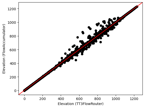
While most of the elevations are quite close, there are some regions with very different elevations. This is due to the different depression finding and routing algorithms, and while the minimum imposition we applied earlier reduces the effect, it does not eliminate it entirely.

fig_tt

Additional references

See also the following citations for more information on Landlab.

• Hobley, D. E. J., Adams, J. M., Nudurupati, S. S., Hutton, E. W. H., Gasparini, N. M., Istanbulluoglu, E. and Tucker, G. E., 2017, Creative computing with Landlab: an open-source toolkit for building, coupling, and exploring two-dimensional numerical models of Earth-surface dynamics, Earth Surface Dynamics, 5(1), p 21-46, doi:10.5194/esurf-5-21-2017.

• Barnhart, K. R., Hutton, E. W. H., Tucker, G. E., Gasparini, N. M., Istanbulluoglu, E., Hobley, D. E. J., Lyons, N. J., Mouchene, M., Nudurupati, S. S., Adams, J. M., and Bandaragoda, C., 2020, Short communication: Landlab v2.0: A software package for Earth surface dynamics, Earth Surf. Dynam., 8(2), p 379-397, doi:10.5194/esurf-8-379-2020.

• Hutton, E., Barnhart, K., Hobley, D., Tucker, G., Nudurupati, S., Adams, J., Gasparini, N., Shobe, C., Strauch, R., Knuth, J., Mouchene, M., Lyons, N., Litwin, D., Glade, R., Giuseppecipolla95, Manaster, A., Abby, L., Thyng, K., & Rengers, F. (2020). landlab [Computer software], doi:10.5281/zenodo.595872.

This paper discusses knickpoint retreat rates in the stream power model

• Berlin, M. M., and R. S.Anderson (2007), Modeling of knickpoint retreat on the Roan Plateau, western Colorado, J. Geophys. Res., 112, F03S06, doi:10.1029/2006JF000553.