Fluvial knickpoints on the Roan Plateau (Python)#
Authors#
Wolfgang Schwanghart, University of Potsdam, FU Berlin (homepage, GitHub) William S. Kearney, University of Potsdam (homepage, GitHub).
This notebook is licensed under CC-BY 4.0.
Highlighted references#
Schwanghart, W., Scherler, D., 2020. Divide mobility controls knickpoint migration on the Roan Plateau (Colorado, USA). Geology, 48 (7), 698–702. [DOI: 10.1130/G47054.1].
Audience#
This is the Jupyter notebook presented at the EGU webinar: Topographic analysis using TopoToolbox in MATLAB and Python. It is suitable for beginners and more advanced users of TopoToolbox.
Introduction#
Fluvial knickpoints, here defined as sharp convexities along river profiles, are important topographic markers indicative of changes in base level of rivers, rock uplift, variations in rock resistance or processes leading to rapid changes in discharge. Here we revisit the Parachute Creek catchment, a basin of the Roan Plateau, that experienced a base level change as the Colorado River rapidly incised 8 Myrs ago (Berlin and Anderson, 2007, Schwanghart and Scherler, 2020). The catchment is steeply dissected by canyons whose heads feature remarkable knickpoints. In this exercise, we will learn to automatically detect these features in longitudinal river profiles, and how they can be used to estimate stream power parameters. To this end, we will use the stream-power incision model to simulate the upstream migration of knickpoints.
Imports#
In Python, we always have to import a few packages including TopoToolbox.
[1]:
import topotoolbox as tt3
import matplotlib.pyplot as plt
from matplotlib.colors import ListedColormap
import numpy as np
from rasterio import CRS
Loading data#
We will use a 30 m DEM of the Roan Plateau obtained from OpenTopography. If you have an OpenTopography API key accessible from the location from which you are running this notebook, you can download the data yourself using load_opentopography. Otherwise, you can acquire the data manually and use read_tif to load the DEM.
[2]:
dem = tt3.load_opentopography(north=39.6960, south=39.3843, west=-108.3168, east=-107.8432, dem_type='COP30')
OpenTopography DEMs are provided in geographic coordinates (latitude-longitude), but TopoToolbox generally prefers to work with projected coordinate systems. We can project into the UTM coordinate system with reproject, using the CRS object from rasterio to supply the desired coordinate system.
[3]:
dem = dem.reproject(CRS.from_epsg(32612), resolution=30.0)
dem.plot_hs(cmap="viridis")
[3]:
<matplotlib.image.AxesImage at 0x7f723d16b800>
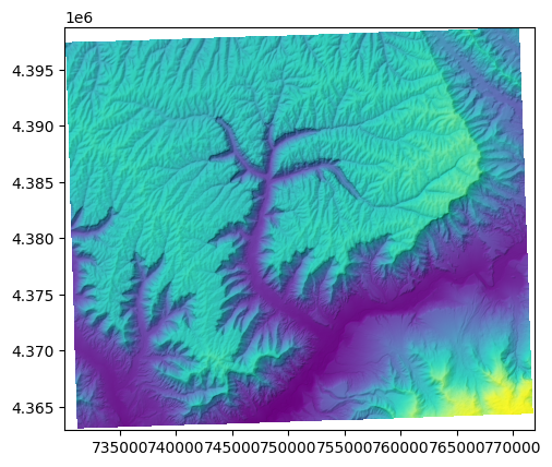
Note the regions of missing data along the edges of the DEM created by the reprojection. TopoToolbox’s analyses can handle those, but it can be a little nicer to crop the DEM to remove those missing data regions and leave a complete rectangular grid. In MATLAB, we use largestinscribedgrid to crop the DEM.
[4]:
dem = dem.largestinscribedgrid()
---------------------------------------------------------------------------
AttributeError                            Traceback (most recent call last)
Cell In[4], line 1
----> 1 dem = dem.largestinscribedgrid()

AttributeError: 'GridObject' object has no attribute 'largestinscribedgrid'
But largestinscribedgrid is not yet implemented in Python. See Issue #437 for more information.
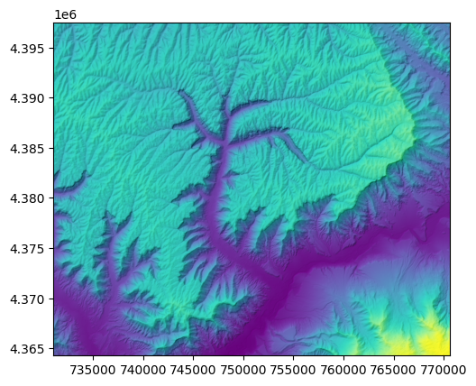
In the meantime, let’s use GridObject.crop. You’ll have to figure out the indices that contain valid data manually, but I’ve done that for you already:
[5]:
dem = dem.crop(bottom=43, top=1151, left=33, right=1352, mode='pixel')
dem.plot_hs(cmap="viridis")
[5]:
<matplotlib.image.AxesImage at 0x7f723cc00230>
Preparing the stream network#
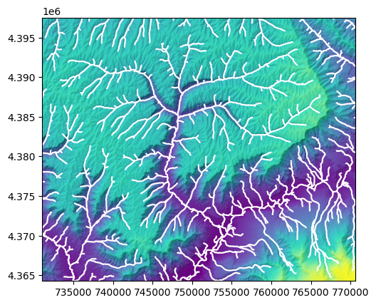
Now that we have a properly referenced DEM, let’s identify the stream network. We’ll use the default flow routing algorithm in TopoToolbox and label stream pixels that have an upstream drainage area of at least 1000 pixels.
[6]:
fd = tt3.FlowObject(dem)
s = tt3.StreamObject(fd, threshold=1000)
[7]:
fig, ax = plt.subplots(1, 1)
dem.plot_hs(cmap="viridis", ax=ax)
s.plot(ax=ax, color="white")
[7]:
<Axes: >
We want to focus our analysis on the Parachute Creek catchment at the center of the DEM and exclude regions that may be influenced by the boundary. We’ll first extract the largest watershed in the DEM, mask out the watersheds touching the boundary, and then clean up the resulting stream network.
[8]:
s = s.klargestconncomps(1)
s = s.removeedgeeffects(fd)
s = s.klargestconncomps(1)

# One could also use `StreamObject.upstreamto`
# if you know the location of the outlet
#
# outlet = np.zeros(fd.shape, dtype=bool)
# outlet[np.unravel_index(1220831, fd.shape)] =  True
# s = s.upstreamto(outlet)
Let’s make a nice map of the Parachute Creek catchment and its stream profile. Identify the drainage basin with FlowObject.drainagebasins and use StreamObject.plotdz to plot the stream profile.
[9]:
db = fd.drainagebasins(outlets=s.stream[s.streampoi('outlets')])
[10]:
fig, (ax1, ax2) = plt.subplots(1, 2, layout="constrained")
db.plot_hs(ax=ax1, elev=dem, cmap=ListedColormap([[0.8, 0.8, 0.8], [0.8*1.0, 0.8*0.62, 0.8*0.47]]))
s.plot(ax=ax1)

s.plotdz(dem, ax=ax2, color='k', linewidth=0.5)
ax2.set_aspect(30)
ax2.set_ylabel("Elevation [m]")
ax2.set_xlabel("Upstream distance [m]")
[10]:
Text(0.5, 0, 'Upstream distance [m]')
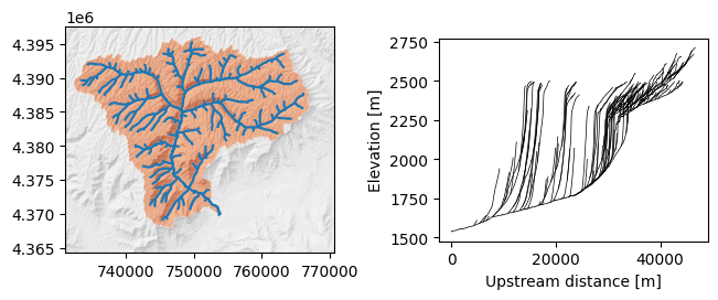
There are many knickpoints in the profile upstream of which the rivers have quite low gradients.
Identify knickpoints#
Now we can use StreamObject.knickpointfinder to identify knickpoints. We can use a fairly large tolerance here because the canyons are steeply incised.
[11]:
kp = s.knickpointfinder(dem, tolerance=100.0)
zs = s.ezgetnal(dem)[kp]
The return value of the knickpointfinder is different from MATLAB. Whereas MATLAB TopoToolbox returns a structure array with information about the knickpoints, pytopotoolbox returns a logical node attribute list. Use that node attribute list to select the information you need, such as the knickpoint elevations (here zs).
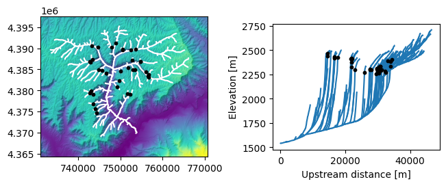
Let’s plot our knickpoints.
[12]:
fig2, (ax1, ax2) = plt.subplots(1, 2, layout="constrained")
dem.plot_hs(cmap="viridis", ax=ax1)
s.plot(ax=ax1, color="white")
ax1.scatter(s.x[kp], s.y[kp], color="black", zorder=2, s=10)

s.plotdz(dem, ax=ax2)
ax2.scatter(s.distance()[kp], zs, color="black", zorder=2, s=10)
ax2.set_aspect(30)
ax2.set_ylabel("Elevation [m]")
ax2.set_xlabel("Upstream distance [m]")
[12]:
Text(0.5, 0, 'Upstream distance [m]')
Chi analysis#
The chi transformation is predicated on the stream-power incision model. The transformation is an integration of the inverse of upstream areas in upstream direction and thereby creates a new distance measure that linearizes the river profile (Perron and Royden 2013). We now calculate the chi transformation of the Parachute Creek using the function chitransform with an mn-ratio of 0.45 and a reference area of 1 sq. km. At a later stage, we will refine the mn-ratio.
[13]:
a = fd.flow_accumulation()
c = s.chitransform(a, a0=1e6, mn=0.45)
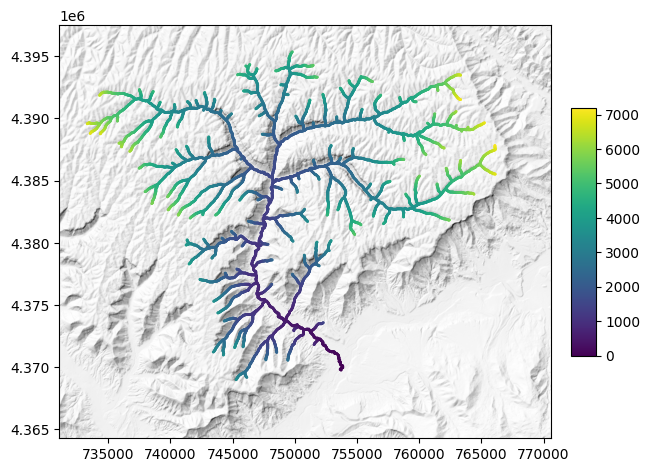
We can plot the results on a map.
[14]:
fig3, ax1  = plt.subplots(1, 1, layout="constrained")

h = dem.hillshade()
h.plot(ax=ax1, cmap="Greys_r")

sm = ax1.scatter(s.x, s.y, c=c, s=1)
cax = ax1.inset_axes([1.04, 0.2, 0.05, 0.6])
fig3.colorbar(sm, cax=cax)
[14]:
<matplotlib.colorbar.Colorbar at 0x7f723cc22cc0>
Modelling spatial patterns of knickpoints using PPS#
We will now use the PPS class to analyze and visualize the knickpoints. PPS means Point Pattern on Stream Networks and is a simple data structure that contains a StreamObject representing the stream network and the locations of the points. Use PPS.from_nal to create a PPS from a logical node attribute list.
[15]:
p = tt3.PPS.from_nal(s, kp)
The PPS functionality in pytopotoolbox is very new. Not all of the functionality of the MATLAB version is available in Python, and many functions behave differently. If you are interested in point pattern analysis and contributing to TopoToolbox, this is a great place to get started!
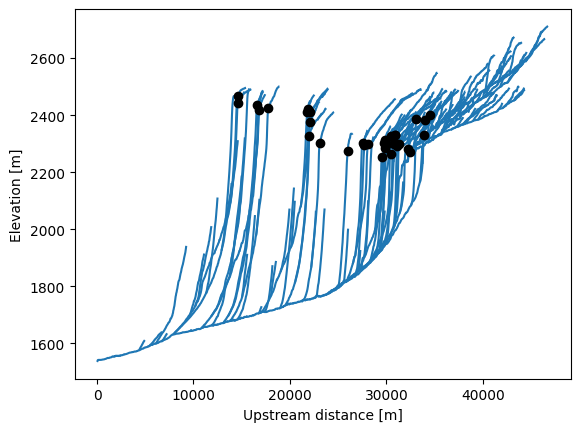
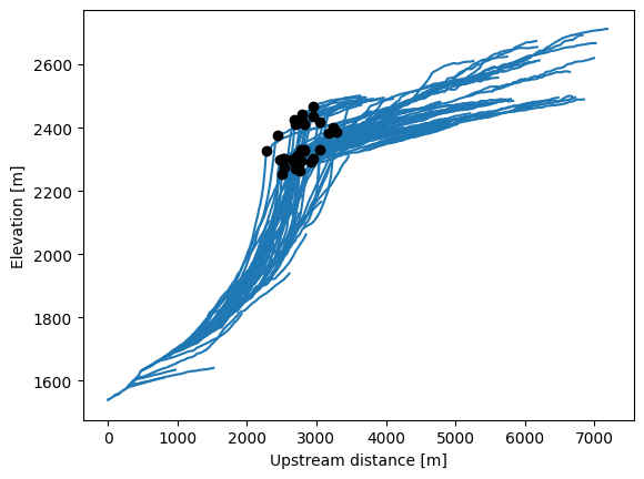
PPS.plotdz will plot the points by upstream distance against elevation, just like StreamObject.plotdz.
[16]:
fig, ax1 = plt.subplots(1, 1)

s.plotdz(dem, ax=ax1)
p.plotdz(dem, ax=ax1, zorder=2, color='k')

ax1.set_xlabel("Upstream distance [m]")
ax1.set_ylabel("Elevation [m]")
[16]:
Text(0, 0.5, 'Elevation [m]')
PPS.rhohat estimates the intensity function of the point pattern, the expected number of points per unit distance, based on a covariate. We compare the intensity functions using upstream distance as the covariate and chi.
[17]:
(x, rho, rhol, rhou) = p.rhohat()
(xc, rhoc, rholc, rhouc) = p.rhohat(covariate=c)
[18]:
fig, (ax1, ax2) = plt.subplots(1, 2, layout="constrained")

ax1.plot(x, rho)
ax1.fill_between(x, rhol, rhou, alpha=0.5)
ax1.eventplot(s.distance()[kp], lineoffsets=0, linelengths=0.05e-3, linewidths=1)
ax1.set_ylabel("Intensity")
ax1.set_xlabel("Upstream distance [m]")

ax2.plot(xc, rhoc)
ax2.fill_between(xc, rholc, rhouc, alpha=0.5)
ax2.eventplot(c[kp], lineoffsets=0, linelengths=0.05e-3, linewidths=1)
ax2.set_ylabel("Intensity")
ax2.set_xlabel("χ")
[18]:
Text(0.5, 0, 'χ')
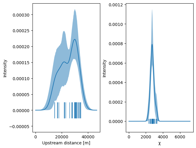
The knickpoints are fairly spread out along the stream network, but the chi transformation collapses them to a narrow range. This is evidence that the knickpoints are derived from a common origin, the base level drop at the catchment outlet.
We can also see this clustering in the stream profiles.
[19]:
fig, ax1 = plt.subplots(1, 1)

s.plotdz(dem, distance=c, ax=ax1)
p.plotdz(dem, distance=c, ax=ax1, zorder=2, color='k')

ax1.set_xlabel("Upstream distance [m]")
ax1.set_ylabel("Elevation [m]")
[19]:
Text(0, 0.5, 'Elevation [m]')
Modelling the knickpoint locations in time#
MATLAB’s PPS functionality includes a set of tools for estimating parameters of the stream power model from the distribution of knickpoints (e.g. mnoptimkp). This has not been implemented in Python yet, in part because we’re unsure how best to integrate this functionality with the Python data analysis ecosystem. This is a great place to get involved if you have some ideas!
Here is a sketch of an implementation using the statsmodels package to fit generalized linear models and scipy to optimize the mn-ratio from the fitted GLM. statsmodels is not included with pytopotoolbox, so you’ll have to install it yourself in your environment. scipy is included with pytopotoolbox.
[20]:
def fitloglinear(p, mn, a, a0=1e6):
    import statsmodels.api as sm

    c = p.s.chitransform(a, a0=a0, mn=mn)
    X = np.stack((np.ones(c.shape), c, c**2)).T

    kp = np.zeros(p.s.stream.size, dtype=bool)
    kp[p.pp] = True

    m = sm.GLM(kp, X, family=sm.families.Binomial())

    return (X, m.fit())

def mnOptim(p, a, a0=1e6):
    from scipy.optimize import minimize_scalar

    f = lambda x: fitloglinear(p, x, a)[1].deviance
    res = minimize_scalar(f, (0.4, 0.45, 0.5), method='brent')
    mn = res.x

    return (mn, fitloglinear(p, mn, a, a0))
[21]:
(mn, (X, res)) = mnOptim(p, a, a0=1e6)

preds = res.predict(X)
d = s.distance("node_to_node")
intensity = preds / np.mean(d)

chimax = -res.params[1]/(2 * res.params[2])

K = chimax/(8e6 * 1e6**mn)
tau = c / (K * 1e6**mn)

mn
[21]:
np.float64(0.44595417669025267)
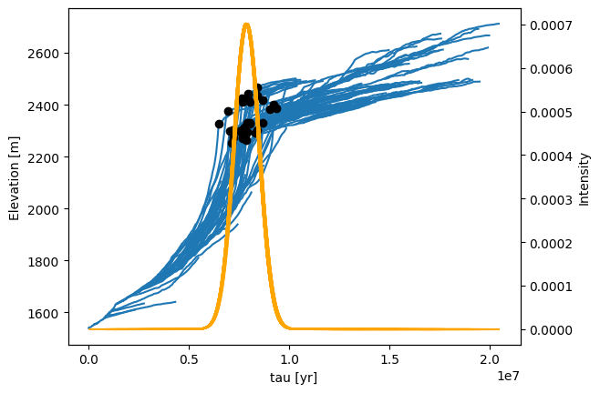
[22]:
fig, ax1 = plt.subplots(1, 1)

s.plotdz(dem, ax=ax1, distance=tau)
p.plotdz(dem, ax=ax1, distance=tau, zorder=2, c='black')

ax1.set_xlabel("tau [yr]")
ax1.set_ylabel("Elevation [m]")

ax2 = ax1.twinx()
s.plotdz(intensity, ax=ax2, distance=tau, color='orange')
ax2.set_ylabel("Intensity")
[22]:
Text(0, 0.5, 'Intensity')
References and Additional Information#
Berlin, M. M. and Anderson, R. S.: Modeling of knickpoint retreat on the Roan Plateau, western Colorado, Journal of Geophysical Research: Earth Surface, 112, https://doi.org/10.1029/2006JF000553, 2007.
Perron, J. T. and Royden, L.: An integral approach to bedrock river profile analysis, Earth Surf. Process. Landforms, 38, 570–576, https://doi.org/10.1002/esp.3302, 2013.
Willett, S. D., McCoy, S. W., Perron, J. T., Goren, L., and Chen, C.-Y.: Dynamic Reorganization of River Basins, Science, 343, 1248765, https://doi.org/10.1126/science.1248765, 2014.