Chi maps of the Rhine-Danube drainage divide (Python)#
Authors#
This notebook is licensed under CC-BY 4.0.
Highlighted references#
Winterberg, S., Willett, S.D. Greater Alpine river network evolution, interpretations based on novel drainage analysis. Swiss J Geosci 112, 3–22 (2019). https://doi.org/10.1007/s00015-018-0332-5
Audience#
New users of pytopotoolbox interested in tectonic geomorphology.
Introduction#
\(\chi\) maps illustrate the potential for dynamic reorganization of river basins (Willett et al., 2014). They display the value of the \(\chi\) metric (Perron and Royden, 2013) at points along the stream network. \(\chi\) is a quantity that arises when solving the one-dimensional steady-state stream power equation by separation of variables. It is given by the equation
where \(A(x)\) is the drainage area at point \(x\) along the stream network. \(A_0\) is a reference drainage area used to nondimensionalize the integrand. \(m\) and \(n\) are constants. The integration is performed upstream from a location denoted \(x_b\).
Winterberg and Willett compute \(\chi\) for the major rivers draining the Alps and interpret maps of \(\chi\) to understand the transient evolution of these river basins in response to tectonics both within and outside of the Alpine orogen. We will replicate a portion of their \(\chi\) analysis, focusing on the drainage divide between the Rhine and Danube river basins.
To compute \(\chi\), we need to
Load a raster containing elevation data
Compute flow directions
Identify the stream network from these drainage directions
Integrate the inverse of the drainage area upstream
Loading data#
We will load a DEM covering the entire Rhine and Danube drainage basins. We will use the SRTM15+ data (Tozer et al. 2019) from OpenTopography. This is a fairly coarse resolution dataset, but it will show the main features in the \(\chi\) map without requiring too much processing time and memory. Try to use a finer dataset like the Copernicus 90 m and compare the results if you are interested.
First, we need to load a few packages including TopoToolbox.
[1]:
import topotoolbox as tt3
import numpy as np # For some additional array operations
import matplotlib.pyplot as plt # For plotting
from rasterio import CRS # To identify the coordinate system that we will project into.
TopoToolbox’s load_opentopography function will download data from OpenTopography.org. You give it a bounding box and the dataset you want to download. You will need an API key from OpenTopography.org for this to work. Once you create an API key, you can either save it as a text file called .opentopography.txt in your home directory or pass it as the api_key argument to
load_opentopography.
[2]:
dem = tt3.load_opentopography(west=3, east=30, south=42, north=53, dem_type='SRTM15Plus')
dem
[2]:
name: OpenTopo_42_53_3_30_SRTM15Plus
        path: /home/runner/.cache/topotoolbox/OpenTopo_42_53_3_30_SRTM15Plus.tif
        rows: 2640
        cols: 6480
        cellsize: 0.004166666666666665
        bounds: BoundingBox(left=2.9999999999999147, bottom=42.00000000000002, right=29.999999999999904, top=53.000000000000014)
        transform: | 0.00, 0.00, 3.00|
| 0.00,-0.00, 53.00|
| 0.00, 0.00, 1.00|
        coordinate system (Geographic): EPSG:4326
        maximum z-value: 4655.0
        minimum z-value: -2887.30615234375
The dem is a GridObject, TopoToolbox’s representation of raster datasets. When displayed a GridObject reports its metadata.
The data returned from OpenTopography is in a geographic coordinate system (latitude and longitude). TopoToolbox works best with data in projected coordinate systems, so we will first reproject the data into the ETRS89 coordinate system, which covers continental Europe. The reproject method on GridObject does this for us. We need to supply the coordinate reference system, so we use the CRS.from_epsg function from the rasterio package and give it the EPSG code for the ETRS89
projection. We also give reproject a resolution to fix the horizontal resolution to 500 m.
[3]:
demr = dem.reproject(CRS.from_epsg(3035),resolution=500.0)
We can visualize this DEM using the GridObject.plot method. We’ll import the cmocean package to give us a nice colormap and pass the norm argument to scale the colors appropriately for this colormap.
[4]:
import cmocean
demr.plot(cmap=cmocean.cm.topo, vmin = -2000, vmax = 2000)
[4]:
<matplotlib.image.AxesImage at 0x7fa42e0edfd0>
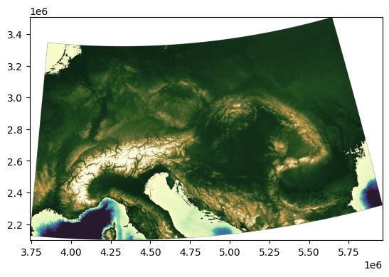
The DEM contains areas below sea level, and one of the assumptions of \(\chi\) analysis is that the stream networks have a common base level at which the upstream integration is started. For simplicity, we will mask out regions with an elevation below 0 m by setting them to NaN, but \(\chi\) analysis can be sensitive to the choice of base level, so it is worth testing your choice of base level.
[5]:
demr.z[demr.z <= 0.0] = np.nan
Identifying the stream network#
Now we are ready to compute the flow directions and the stream network. TopoToolbox represents flow directions using a FlowObject and stream networks with a StreamObject. Create the former by giving it the reprojected and masked DEM.
[6]:
fd = tt3.FlowObject(demr)
And then create a StreamObject with the FlowObject by defining streams as pixels with a minimum drainage area of \(10\ \mathrm{km^2}\).
[7]:
s = tt3.StreamObject(fd, units='km2', threshold=10.0)
This stream network covers the entire DEM, so we restrict it to the Rhine and Danube by using the klargestconncomps method to select the two largest drainage basins. This works because the Rhine and Danube happen to be the two largest basins in the DEM. If you wanted to select different basins (such as the Po and Rhône as in Winterberg and Willett), you would need some more complicated logic here.
[8]:
s = s.clean().klargestconncomps(2)
Computing \(\chi\)#
The \(\chi\) transform integrates the inverse of the upstream area, so we first need to compute the upstream area. The FlowObject.flow_accumulation method does this.
[9]:
a = fd.flow_accumulation()
And finally, we compute \(\chi\) with the StreamObject.chitransform method. We give it the drainage area raster and parameters setting the ratio \(m/n = 0.45\) and the reference drainage area \(A_0 = 1\ \mathrm{m^2}\). These are the parameters given by Winterberg and Willett.
The units of the drainage area raster are in pixels by default. We can correct that by multiplying the drainage area raster by the square of the cellsize, but chitransform will do it for us if we pass correctcellsize=True.
[10]:
c = s.chitransform(a, mn=0.45, a0=1.0, correctcellsize=True)
The array c contains the \(\chi\) values for every point in our stream network.
Plotting the results#
To visualize the results, we will plot c in a map view colored by \(\chi\). First, we need some more plotting libraries. These are all included with matplotlib but are not imported by the import matplotlib.pyplot as plt we did earlier.
[11]:
from matplotlib.colors import ListedColormap, Normalize, LogNorm
from matplotlib.patches import Patch
from mpl_toolkits.axes_grid1 import make_axes_locatable
from matplotlib.ticker import FuncFormatter
First, we will identify the two drainage basins. The FlowObject.drainagebasins method can do this for us, but it will label all of the basins in the DEM, and we would then have to pick out the Rhine and Danube basins from the results. We can do this on our own by picking out the outlets of the Rhine and Danube from our StreamObject, labeling them with the numbers 1 and 2, and then filling in the rest of the drainage basin with the propagatevaluesupstream_i64 function.
[12]:
outlets = s.streampoi('outlets')

db = np.zeros(s.shape, dtype=np.int64, order=fd.order)
db = demr.duplicate_with_new_data(db)

db[s.node_indices] = np.cumsum(outlets)
tt3._stream.propagatevaluesupstream_i64(db, fd.source, fd.target)
Our plot is going to focus on the divide between the Rhine and Danube drainage basins. To avoid plotting data outside this region, which can be very slow, we will crop our DEM and drainage basin rasters to the region of interest.
[13]:
bounds = [4100000, 4400000, 2600000, 2900000]

dbc = db.crop(left=bounds[0], right=bounds[1], bottom=bounds[2], top=bounds[3], mode='coordinate')
demc = demr.crop(left=bounds[0], right=bounds[1], bottom=bounds[2], top=bounds[3], mode='coordinate')
We will also filter the StreamObject so it only includes points within this bounding box. The StreamObject.subgraph method takes an array that is True for all nodes in the original StreamObject that you want in the new one. We also use this filter array to select the corresponding \(\chi\) values.
[14]:
x, y = s.coordinates
filt = (bounds[0] <= x) & (x < bounds[1]) & (bounds[2] <= y) & (y < bounds[3])

sc = s.subgraph(filt)
cc = c[filt]
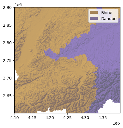
Now we are ready to make our plot. First, we’ll plot the hillshade of the drainage basins using the plot_hs method on the cropped drainage basin raster. We give it the cropped DEM as the elev argument and set the colormap as well. I have picked a couple of colors for the drainage basins that won’t interfere too much with the colors of the \(\chi\) values that we’ll add in a moment.
[15]:
fig, ax = plt.subplots(1,1)

basin_colors = {
    'Rhine' : (0.45, 0.25, 0.00),
    'Danube': (0.18, 0.10, 0.40),
}

db_alpha = 0.6
legend_elements = [
    Patch(facecolor=basin_colors['Rhine'], label='Rhine', alpha=db_alpha),
    Patch(facecolor=basin_colors['Danube'], label='Danube', alpha=db_alpha),
]

dbc.plot_hs(ax=ax, elev=demc,
           cmap=ListedColormap([(1.0, 1.0, 1.0), basin_colors['Rhine'], basin_colors['Danube']]),
           alpha=db_alpha, exaggerate=10)

ax.legend(handles=legend_elements, loc='upper right')
[15]:
<matplotlib.legend.Legend at 0x7fa42e197fe0>
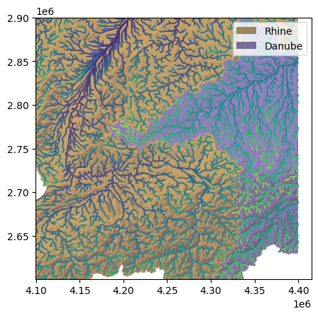
We plot the stream network as a colored scatter plot. The StreamObject.x and StreamObject.y properties give the x and y coordinates of every node in the stream network.
At this scale the separation between the points is not visible, but you might like to plot the stream network as connected lines. The StreamObject.plot method will do this for you, but, unfortunately, adding the colors is somewhat more complicated, so we’ll stick with the scatter plot for now.
[16]:
cmap = plt.cm.viridis
norm = plt.Normalize(vmin=0.0, vmax=45.0)
ax.scatter(sc.x + 0.5*sc.cellsize, sc.y + 0.5*sc.cellsize, c=cc, s=0.1, cmap=cmap, norm=norm)

fig
[16]:
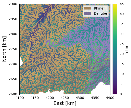
Finally, we will add a colorbar and some nice axis labels.
[17]:
divider = make_axes_locatable(ax)
cax = divider.append_axes("right", size="5%", pad=0.1)

cb = fig.colorbar(plt.cm.ScalarMappable(norm=norm, cmap=cmap), cax=cax)
cb.set_label(label='χ [m]')

km_formatter = FuncFormatter(lambda x, pos: f'{x/1000:.0f}')
ax.xaxis.set_major_formatter(km_formatter)
ax.yaxis.set_major_formatter(km_formatter)

ax.set_xlabel("East [km]", size=14)
ax.set_ylabel("North [km]", size=14)
ax.set_xlim(4100000, 4400000)
ax.set_ylim(2600000, 2900000)

fig
[17]:

We can easily see from our \(\chi\) map the main feature of the Rhine-Danube divide identified by Winterberg and Willett: the \(\chi\) values are much higher in the Danube basin than in the Rhine. The relatively shallower gradients of the Danube are reflected in this asymmetry, which suggests that the drainage divide will migrate into the Danube basin, shrinking it while the Rhine basin grows.
Quantitative comparison with MATLAB#
The MATLAB counterpart to this notebook conducts the same analysis using TopoToolbox in MATLAB. If you would like to see how the two packages compare, run the MATLAB Live Script. It will save its results in a text file called chiplot.txt. If you are running this from the gallery Git repository, you can find it at the following location. Otherwise change the filename below to wherever the chiplot file is located.
The dataset contains the elevation and \(\chi\) values as well as the drainage basin labels for pixels in the main trunks of the Rhine and Danube in a comma-separated value file. Load this with the loadtxt function from numpy.
[18]:
zm, cm, dbm = np.loadtxt("../../matlab/alpine-chimaps/chiplot.txt",delimiter=',').T
We would normally plot elevation against \(\chi\) using the StreamObject.plotdz method, but because the connectivity information is not saved, we’ll make our own plot. We have to sort the MATLAB data by \(\chi\) for this to work correctly.
[19]:
idxs = np.argsort(cm)
zm = zm[idxs]
cm = cm[idxs]
dbm = dbm[idxs]
Now we compute the same information from our StreamObject in Python. We compute the trunks and then filter them to the portion of the streams greater than 250 m.
[20]:
st = s.trunk()
stt = st.subgraph(st.ezgetnal(demr) >= 250)
cp = np.zeros(s.shape)
cp[s.node_indices] = c
ztt = stt.ezgetnal(demr)
ctt = stt.ezgetnal(cp)
dbt = stt.ezgetnal(db)

idxs = np.argsort(ctt)
ztt = ztt[idxs]
ctt = ctt[idxs]
dbt = dbt[idxs]
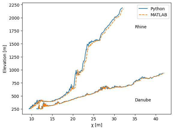
[21]:
fig2, ax2 = plt.subplots()
ax2.plot(ctt[dbt==1], ztt[dbt==1], color="tab:blue", linestyle="solid", label="Python")
ax2.plot(cm[dbm==1], zm[dbm==1], color="tab:orange", linestyle="dashed", label="MATLAB")

ax2.plot(ctt[dbt==2], ztt[dbt==2], color="tab:blue", linestyle="solid")
ax2.plot(cm[dbm==2], zm[dbm==2], color="tab:orange", linestyle="dashed")

ax2.set_ylabel("Elevation [m]")
ax2.set_xlabel("χ [m]")

ax2.annotate("Rhine", xy=(35, 1800))
ax2.annotate("Danube", xy=(35, 400))

ax2.legend()
[21]:
<matplotlib.legend.Legend at 0x7fa42bfe87d0>
Additional References#
Tozer, B, Sandwell, D. T., Smith, W. H. F., Olson, C., Beale, J. R., & Wessel, P. (2019). Global bathymetry and topography at 15 arc sec: SRTM15+. Distributed by OpenTopography. https://doi.org/10.5069/G92R3PT9. Accessed 2026-04-21
Perron, J.T. and Royden, L. (2013), An integral approach to bedrock river profile analysis. Earth Surf. Process. Landforms, 38: 570-576. https://doi.org/10.1002/esp.3302
[22]:
fig
[22]: