An introduction to TopoToolbox

Welcome to the TopoToolbox Gallery, a collection of user-contributed demonstrations of TopoToolbox!

To begin, we will create a hillshade of a digital elevation model of Big Tujunga creek in California. Start by importing topotoolbox and pyplot.

import topotoolbox as tt3
import matplotlib.pyplot as plt

The Big Tujunga DEM is provided as one of the example DEMs with TopoToolbox, so we can load it using the load_dem function.

dem = tt3.load_dem('bigtujunga')
dem

name: bigtujunga
        path: /home/runner/.cache/topotoolbox/bigtujunga.tif
        rows: 643
        cols: 1197
        cellsize: 30.0
        bounds: BoundingBox(left=376313.6554542635, bottom=3788627.8276283755, right=412223.6554542635, top=3807917.8276283755)
        transform: | 30.00, 0.00, 376313.66|
| 0.00,-30.00, 3807917.83|
| 0.00, 0.00, 1.00|
        coordinate system (Projected): EPSG:32611
        maximum z-value: 2295.0
        minimum z-value: 315.0

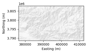
The DEM is returned as a GridObject, TopoToolbox’s representation of single-band raster datasets. To make a hillshade, we can use the plot_hs method on the GridObject. Instead of using TopoToolbox’s default colormap, we’ll use the ListedColormap from matplotlib’s colors module to produce a greyscale hillshade. We give it a single color of light grey to represent the lightest value, and plot_hs takes care of shading the rest of the DEM. Increasing the vertical exaggeration a little, makes the relief more apparent.

from matplotlib.colors import ListedColormap

fig = plt.figure(layout='constrained')
ax1 = plt.subplot(121)
dem.plot_hs(ax=ax1, cmap=ListedColormap([0.9, 0.9, 0.9]), exaggerate=3)

ax1.set_xlabel("Easting (m)")
ax1.set_ylabel("Northing (m)")

Text(0, 0.5, 'Northing (m)')

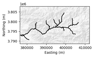
Now let’s add a visualization of the stream network to this map. We first create a FlowObject storing flow directions on the DEM, and then a StreamObject that picks out the streams. We call the klargestconncomps method on the StreamObject to restrict our analysis to the main watershed.

fd = tt3.FlowObject(dem)
s  = tt3.StreamObject(fd).klargestconncomps(1)

We can add the StreamObject to our plot with its plot method.

s.plot(ax=ax1, color="black")
fig

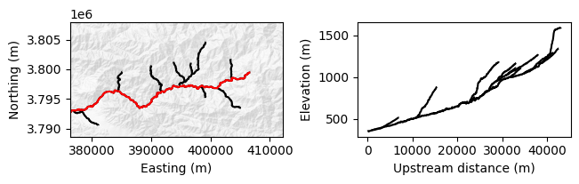
Finally, let’s use the trunk method on the StreamObject to pick out the longest stream in the watershed, and the plotdz method to plot its profile in another subplot.

t = s.trunk()
t.plot(ax=ax1, color="red")

ax2 = fig.add_subplot(122, box_aspect=643/1197)
s.plotdz(dem, ax=ax2, color="black")
ax2.set_xlabel("Upstream distance (m)")
ax2.set_ylabel("Elevation (m)")

fig