Graphflood complete overview#
Quickstart, convergence checking and boundary condition handling#
Authors#
Boris Gailleton, Université de Rennes Homepage
This notebook is licensed under CC-BY 4.0.
Highlighted references#
graphflood (Gailleton et al., 2024) simulates how water moves across terrain surfaces using a fast 2D stationary diffusive wave approximation.
Audience#
pytopotoolbox users, interested in fast stationary flow approximations (2D flow depth and velocity).
Introduction#
High-resolution DEMs often contain rivers that are several pixels wide, making them difficult to represent with classic steepest-descent routing algorithms. Similarly, estimating river geometry across multiple hydrological states typically requires solving the shallow water equations.
While accurate, shallow water solvers are computationally expensive, especially when only first-order estimates of hydraulic metrics are needed rather than a complete hydrograph simulation.
Steady-state solvers such as GraphFlood, Floodos, and FastFlood provide a faster alternative. Instead of simulating the full transient evolution of a flood (e.g., dam-break wave propagation), they directly compute the equilibrium flow field.
Given:
a digital elevation model (DEM),
water inputs (rainfall or prescribed inflow),
these models iteratively route water until they reach a steady state and produce maps of:
Dynamic Metric |
Variable |
|---|---|
Flow depth |
\(h\) |
Velocity |
\(u\) |
Shear stress |
\(\tau\) |
Discharge |
\(Q\) |
Prerequisites#
Install dependencies via your terminal:
pip install topotoolbox
pip install ipympl # Optional: For interactive figures
Offline assistance?#
Last resort: drop me an email (boris.gailleton@univ-rennes.fr)
[1]:
# General imports
import topotoolbox as ttb
import matplotlib.pyplot as plt
import numpy as np
import time
import scipy.stats as st
from scipy.ndimage import binary_closing, distance_transform_edt
from skimage.morphology import skeletonize

# Set matplotlib backend
%matplotlib inline
## If you want interactive plots
# %matplotlib ipympl
---------------------------------------------------------------------------
ModuleNotFoundError                       Traceback (most recent call last)
Cell In[1], line 8
      4 import numpy as np
      5 import time
      6 import scipy.stats as st
      7 from scipy.ndimage import binary_closing, distance_transform_edt
----> 8 from skimage.morphology import skeletonize
      9
     10 # Set matplotlib backend
     11 get_ipython().run_line_magic('matplotlib', 'inline')

ModuleNotFoundError: No module named 'skimage'
Quickstart#
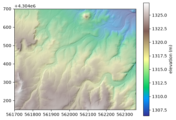
Provide a raw DEM and your water inputs to calculate balanced flow conditions and track fluid behavior maps instantly.
[2]:
# Load DEM and crop to a specific spatial subset via percentage thresholds
dem = ttb.load_dem('greenriver')
dem = dem.crop(0.35, 0.68, 0.3, 0.85, 'percent')

# if you want to load your DEM:
# dem = ttb.read_tif('mydem.tif')

# Plot the cropped topography with an overlaid hillshade
fig, ax = plt.subplots()
cb = ax.imshow(dem.z, cmap='terrain', extent=dem.extent)
ax.imshow(dem.hillshade(), cmap='gray', extent=dem.extent, alpha=0.6)
plt.colorbar(cb, label='elevation (m)')
plt.show()
GFObject (Graphflood Object)#
The primary interface utilized to initialize and run the graphflood engine.
Argument |
Requirement |
Description |
|---|---|---|
grid |
|
Core topography/DEM input grid layout. |
bcs |
|
Pixel boundary condition codes. Defaults to unconstrained borders. |
p |
|
Precipitation supply rates (scalar value or 2D array matrix in \(m/s\)). |
manning |
|
Manning surface roughness index (\(n\)) used during flow calculations. |
[3]:
# Instantiate the Graphflood object with 100 mm/h uniform precipitation converted to m/s
## 100 mm/h is super high, I chose it to make sure even in our v. small demo site we generate enough flooding
gfo = ttb.GFObject(dem, p=(100e-3)/3600, manning=0.05)
Running the Model#
The solver routes surface water incrementally across cells until it settles into equilibrium.
Control Parameter |
Impact on Convergence |
Constraint / Risk |
|---|---|---|
Iterations |
Higher execution runs bring the solver closer to true mathematical flow alignment. |
Increases computational compute time. |
Time Step ( |
Larger steps speed up convergence rates towards a steady-state layout. |
Excessive values trigger numerical instability and cause solution degradation. |
Key Distinction: The parameter
dtfunctions purely as a mathematical tuning knob to speed up calculations. It does not reflect actual physical timeline tracking.
[4]:
# Run the steady-state solver loop for 100 fixed steps
gfo.run_n_iterations(dt=1e-2, n_iterations=100)
[5]:
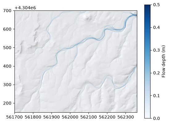
# Display calculated water depths layered over the relief hillshade
fig, ax = plt.subplots()
cb = ax.imshow(gfo.hw, cmap='Blues', extent=dem.extent, vmax=0.5)
ax.imshow(dem.hillshade(), cmap='gray', extent=dem.extent, alpha=0.4)
plt.colorbar(cb, label='Flow depth (m)')
plt.show()
Computed Metrics#
Shear Stress (\(\tau\))#
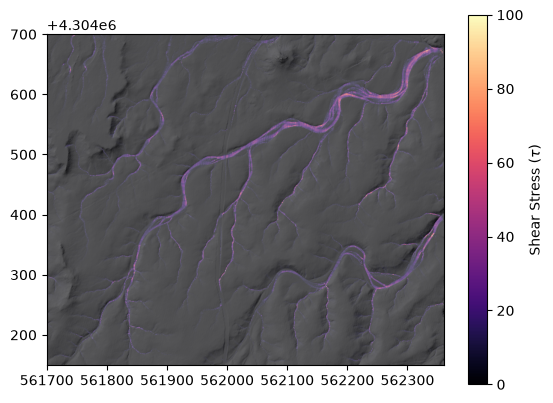
The total dragging friction force exerted by shifting water directly along the surface channel bed.
Engine Execution: Extracted directly using
gfo.compute_tau()based on calculated local depth (\(h\)) and hydraulic water surface slope profiles (\(S_w\)).
[6]:
# Compute and map boundary shear stress across the channel bed
shear_stress = gfo.compute_tau()

#
fig, ax = plt.subplots()
cb = ax.imshow(shear_stress, cmap='magma', extent=dem.extent, vmax=100)
ax.imshow(dem.hillshade(), cmap='gray', extent=dem.extent, alpha=0.4)
plt.colorbar(cb, label=r'Shear Stress ($\tau$)')
plt.show()
Flow Velocity#
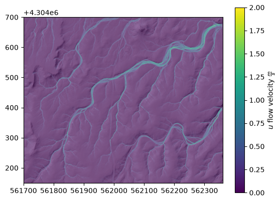
Calculates flow velocity magnitudes (\(u\)) across your target grid landscape layout.
Execution:
gfo.get_u()Roadmap: Directional vector component tracking layouts will follow in an upcoming update.
[7]:
# Retrieve depth-averaged flow velocity magnitudes
flow_velocity = gfo.get_u()

fig, ax = plt.subplots()
cb = ax.imshow(flow_velocity, cmap='viridis', extent=dem.extent, vmax = 2.)
ax.imshow(dem.hillshade(), cmap='gray', extent=dem.extent, alpha=0.4)
plt.colorbar(cb, label=r'$u$ flow velocity $\frac{m}{s}$')
plt.show()
Discharge & Hydraulic Slope#
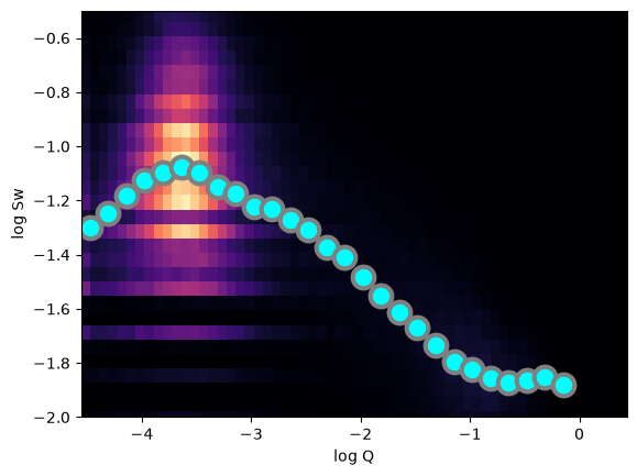
A custom hydraulic twist on classical geomorphic slope-area plotting, replacing upstream drainage basin surface area (\(A\)) with explicitly calculated flow discharge tracking values (\(Q\)).
Core Objective: Compares log-scaled surface slope records (\(S_w\)) against discharge rates (\(Q\)) to distinguish distinct flow channels and landscape scaling domains.
[8]:
# Flatten volumetric discharge and hydraulic water surface slope grids into log space
Q_in = np.log10(gfo.get_qvol_i().z.ravel())
Sw = np.log10(gfo.get_sw().z.ravel())

# Filter out NaN and infinite elements
mask = np.isfinite(Q_in) & np.isfinite(Sw)
Q_in = Q_in[mask]
Sw = Sw[mask]

# 1. Compute 2D Density (Binned Counts)
bins2D = 60
stat_2d, x_edges, y_edges, _ = st.binned_statistic_2d(Q_in, Sw, None, 'count', bins=bins2D)
#
# 2. Compute 1D Profile (Median of Y binned by X)
bins = 30
bin_means, bin_edges, _ = st.binned_statistic(Q_in, Sw, statistic='median', bins=bins)
bin_centers = (bin_edges[:-1] + bin_edges[1:]) / 2

# 3. Plot
fig, ax = plt.subplots()

# 2D Density Map distribution
ax.imshow(stat_2d.T, origin='lower', cmap='magma', aspect='auto',
               extent=[x_edges[0], x_edges[-1], y_edges[0], y_edges[-1]])

# 1D Overlaid Median Line trend line
ax.scatter(bin_centers, bin_means, facecolor='cyan', edgecolor='gray', lw=3, s=200)

ax.set_ylim(-2, -0.5)
ax.set_xlabel('log Q')
ax.set_ylabel('log Sw')
plt.show()
/tmp/ipykernel_23689/4067809772.py:2: RuntimeWarning: divide by zero encountered in log10
  Q_in = np.log10(gfo.get_qvol_i().z.ravel())
/tmp/ipykernel_23689/4067809772.py:3: RuntimeWarning: divide by zero encountered in log10
  Sw = np.log10(gfo.get_sw().z.ravel())
[9]:
# Initialize empty mask grid matching the topography geometry
domain = np.zeros_like(dem.z)
#
text_arrays = """
Extract raw arrays for discharge and water surface slopes
"""
Qi2d = np.log10(gfo.get_qvol_i().z)
Sw2d = np.log10(gfo.get_sw().z)
#
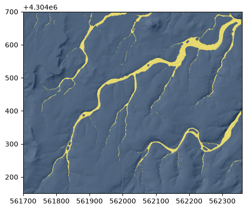
# Isolate channel cells using joint flow thresholds
domain[(Qi2d > -1.7) & (Sw2d < -1.4) & (gfo.hw.z > 0.05)] = 1
# Clean up gaps and edge noise via morphological binary closing operations
domain = binary_closing(domain, iterations=3)
#
# Visualize the calculated binary river network mask
fig, ax = plt.subplots()
cb = ax.imshow(domain, cmap='cividis', extent=dem.extent)
ax.imshow(dem.hillshade(), cmap='gray', extent=dem.extent, alpha=0.4)
plt.show()
/tmp/ipykernel_23689/1927711354.py:7: RuntimeWarning: divide by zero encountered in log10
  Qi2d = np.log10(gfo.get_qvol_i().z)
/tmp/ipykernel_23689/1927711354.py:8: RuntimeWarning: divide by zero encountered in log10
  Sw2d = np.log10(gfo.get_sw().z)
Automated Channel Width Extraction#
A clean, efficient post-processing workflow executed entirely via standard scipy and scikit-image sequences to map true channel width paths straight from our 2D hydraulic footprint.
Reference Code: Review the complete original script logic inside the official TopoToolbox Paper Gallery Notebook.
Processing Pipeline#
Step |
Operation |
Core Target Function |
|---|---|---|
1 |
Clean Channel Mask |
Isolate active river zones (based on slope-discharge limits) and remove interior holes using |
2 |
Extract Centerline Spines |
Thin the continuous 2D mask tracks down into an individual 1-pixel wide skeleton network via |
3 |
Calculate Edge Distance |
Compute exact Euclidean coordinate distances from centerline nodes to the nearest boundary edge using |
[10]:
# =============================================================================
# 1. MORPHOLOGICAL ANALYSIS & DISTANCE TRANSFORM
# =============================================================================

# Map the exact Euclidean distance from every channel pixel to the nearest dry bank boundary
dt_edt = distance_transform_edt(domain)

# Thin the 2D binary channel mask down to a continuous, 1-pixel wide centerline network
skel = skeletonize(domain)


# =============================================================================
# 2. CHANNEL WIDTH COMPUTATION & FILTERING
# =============================================================================

# Calculate absolute physical channel width (m) along the centerline skeleton
# Formula tracks full-width (2 * half-width) and adjusts for discrete pixel resolution
width = 2 * dt_edt[skel] * dem.cellsize - dem.cellsize

# Generate a boolean filtering mask to isolate features >= 2 meters wide
mask = width >= 2


# =============================================================================
# 3. SPATIAL COORDINATE TRANSFORMATION
# =============================================================================

# Extract the 2D array matrix row and column indices for all skeleton nodes
rows_skel, cols_skel = np.where(skel)

# Project pixel index positions into true geographic map coordinates (X, Y)
xskel, yskel = ttb.transform_coords(
    dem,
    rows_skel,
    cols_skel,
    input_mode='indices2D',
    output_mode='coordinates'
)


# =============================================================================
# 4. GEOGRAPHIC VISUALIZATION
# =============================================================================

fig, ax = plt.subplots()

# Base Layer: Render the topography hillshade in grayscale
ax.imshow(dem.hillshade(), cmap='gray', extent=dem.extent, vmax=1.2)
ax.imshow(domain, cmap='cividis', extent=dem.extent, alpha=0.25)

# Data Overlay: Plot the filtered centerline coordinates colored by calculated width
cb = ax.scatter(
    xskel[mask],
    yskel[mask],
    lw=0,
    c=width[mask],
    cmap='plasma'
)

# Render colorbar interface and output graphic area
plt.colorbar(cb, label='width (m)')
plt.show()
---------------------------------------------------------------------------
NameError                                 Traceback (most recent call last)
Cell In[10], line 9
      5 # Map the exact Euclidean distance from every channel pixel to the nearest dry bank boundary
      6 dt_edt = distance_transform_edt(domain)
      7
      8 # Thin the 2D binary channel mask down to a continuous, 1-pixel wide centerline network
----> 9 skel = skeletonize(domain)
     10
     11
     12 # =============================================================================

NameError: name 'skeletonize' is not defined
Done with the Quickstart#
Checking If the Model Is Done (Convergence)#
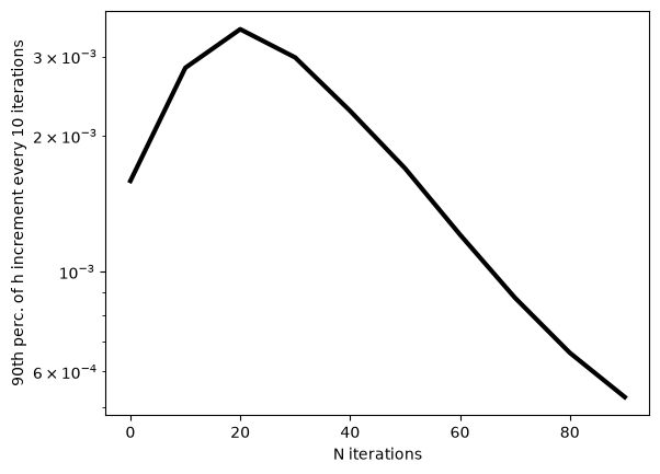
How can we verify when the simulation has finished its job? We track our system metrics to find where local water levels stop changing and lock down into a stable state.
What We Check |
Ideal Goal |
What Actually Happens |
|---|---|---|
Water Balance |
Water In = Water Out (\(Q_{in} = Q_{out}\)) |
The total volume exiting map parameters will slowly approach absolute parity with inflow records over time. |
Stable Water Depth |
Depth stops changing (\(\frac{dh}{dt} = 0\)) |
While water depths rarely freeze completely to absolute zero change, grid values level off enough to stop mattering very quickly. |
Quick Troubleshooting Strategy#
Run it longer: If water surfaces are actively moving, extend processing loops using standard calls to
gfo.run_n_iterations(...).Best way to check: Monitor the structural changes in depth profile maps between cycles (\(dh\)). Once variance adjustments shrink past a nominal target baseline, your model is balanced.
[11]:
# Re-instantiate model instance to benchmark step-wise iteration increments
gfo = ttb.GFObject(dem, p=100e-3/3600, manning=0.05)
dhs = [gfo.hw.z.copy()]
[12]:
#
N = 10
N_it = 10
# Stepwise solver tracking loop to monitor water depth grid adjustments over execution
for i in range(N):
    print(f'running {(i+1) * N_it}/{N * N_it}', end='\r', flush=True)
    gfo.run_n_iterations(dt=5e-2, n_iterations=N_it)
    # Enforce boundary zero-depth conditions at perimeter edges
    gfo.hw[[0, -1], :] = 0
    gfo.hw[:, [-1, 0]] = 0
    dhs.append(gfo.hw.z.copy())
dhs_arr = np.array(dhs)
running 100/100
[13]:
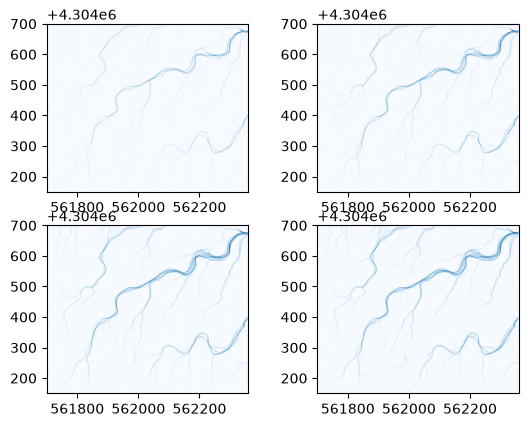
# Close any lingering plots and check depth distribution snapshots at steps 1, 2, 5, 10
# plt.close('all')
fig, axes = plt.subplots(2, 2)
cb = axes[0, 0].imshow(dhs_arr[1], cmap='Blues', extent=dem.extent, vmax=0.5)
cb = axes[0, 1].imshow(dhs_arr[2], cmap='Blues', extent=dem.extent, vmax=0.5)
cb = axes[1, 0].imshow(dhs_arr[5], cmap='Blues', extent=dem.extent, vmax=0.5)
cb = axes[1, 1].imshow(dhs_arr[10], cmap='Blues', extent=dem.extent, vmax=0.5)
plt.show()
[14]:
# Plot the log-scaled progression of the 90th percentile depth variance delta to assess convergence
# plt.close('all')
fig, ax = plt.subplots()
ax.plot(np.arange(len(dhs)-1)*N_it, np.percentile(np.abs(np.diff(dhs_arr, axis=0)), 90, axis=(1, 2)), lw=3, color='k')
ax.set_xlabel('N iterations')
ax.set_ylabel(f'90th perc. of h increment every {N_it} iterations')
ax.set_yscale('log')
time.sleep(0.2) # Mitigation step preventing rendering race condition bugs inside JupyterLab interface
plt.show()
Boundary Conditions: The “Reach” Case#
Isolate explicit river paths by defining routing directions: driving inbound stream channels through a selected boundary zone (South) and establishing exit points along another (North).
Boundary Condition (BC) Grid Codes#
Pixel actions are set using an integer array layer that exactly mirrors our topography layout geometry:
BC Code |
Type |
Flow Behavior |
|---|---|---|
|
No Data / Wall |
Solid impermeable boundary. Flow is completely blocked and cannot pass or exit. |
|
Normal Active Area |
Standard interior routing. Flow moves continuously across cells but cannot scale over borders. |
|
Outlet Gate |
Unconstrained drainage point. Flow permanently empties out of the simulation at this node. |
Critical Rule: Active simulation runs require at least one pixel configured as an outlet gate (
3). If an exit path is missing, water pools infinitely and the solver cannot balance metrics.
Spatial Input Mapping (Point Source Discharge)#
Instead of applying uniform rainfall across the entire map footprint, we switch to a spatially variable input array. This zeroes out fluid additions everywhere except at our designated channel source node, precisely replicating a localized upstream stream inflow.
[15]:
# Set default processing mask states to internal routing (1)
bcs = np.ones_like(dem.z, dtype=np.uint8)
# Impose solid impermeable boundaries (0) around the immediate exterior rows and columns
bcs[[-1, 0], :] = 0
bcs[:, [-1, 0]] = 0

# Construct empty array map to manage explicit flow source locations
prec_in = np.zeros_like(dem.z, dtype=np.float32)

# Draw background reference surface map
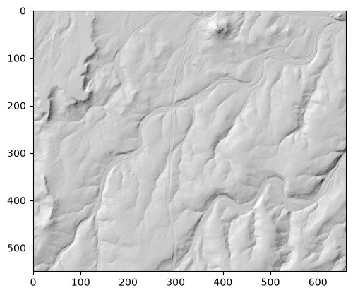
fig, ax = plt.subplots()
ax.imshow(dem.hillshade(), cmap='gray')
plt.show()
[16]:
# Create an unconstrained drainage exit point (3) on a segment of the boundary wall
bcs[20:50, -1] = 3

# Inject a localized discharge point source of 5 m3/s scaled to a precipitation equivalent flux
prec_in[-2, 30] = 5 / (dem.cellsize**2)
[17]:
# Draw background reference surface map
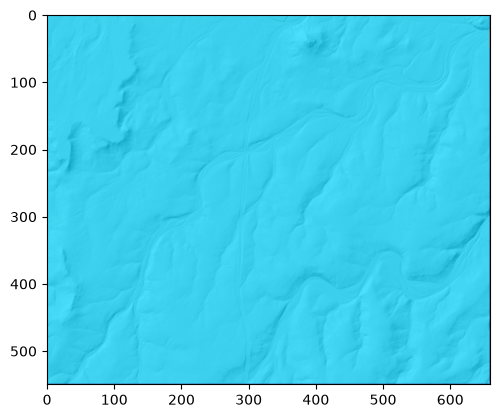
fig, ax = plt.subplots()
ax.imshow(dem.hillshade(), cmap='gray')
ax.imshow(bcs, cmap='jet', alpha = 0.7)
plt.show()
[18]:
# Initialize a new Graphflood model configuration using the boundary matrix and localized flow input
gfo = ttb.GFObject(dem, p=prec_in, manning=0.05, bcs=bcs)
[19]:
# Execute processing loop and mask out non-contributing dry terrain nodes
gfo.run_n_iterations(dt=1e-2, n_iterations=100)
gfo.hw.z[gfo.get_qvol_i().z == 0] = 0.
[20]:
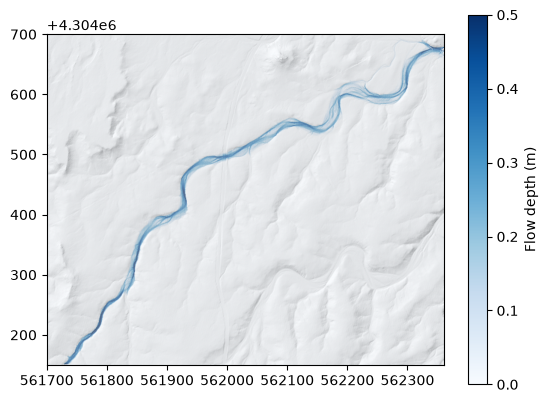
# View inundation track profile resulting from the isolated reach boundary settings
fig, ax = plt.subplots()
cb = ax.imshow(gfo.hw, cmap='Blues', extent=dem.extent, vmax=0.5)
ax.imshow(dem.hillshade(), cmap='gray', extent=dem.extent, alpha=0.4)
plt.colorbar(cb, label='Flow depth (m)')
plt.show()
[21]:
# Archive current water depth output, scale point discharge by 10x, and update flow fields
thw = gfo.hw.z.copy()
gfo.precipitations = prec_in * 10
gfo.run_n_iterations(dt=1e-3, n_iterations=100)
gfo.hw.z[gfo.get_qvol_i().z == 0] = 0.
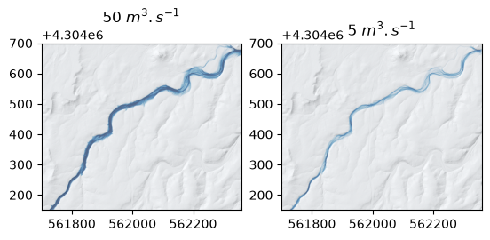
[22]:
# Compare flow depth signatures between the 5 m3/s and 50 m3/s discharge inputs side-by-side
fig, axes = plt.subplots(1, 2)
axes[0].imshow(gfo.hw, cmap='Blues', extent=dem.extent, vmax=0.5)
axes[1].imshow(thw, cmap='Blues', extent=dem.extent, vmax=0.5)
axes[0].imshow(dem.hillshade(), cmap='gray', extent=dem.extent, alpha=0.4)
axes[1].imshow(dem.hillshade(), cmap='gray', extent=dem.extent, alpha=0.4)

axes[0].set_title(r'50 $m^3.s^{-1}$')
axes[1].set_title(r'5 $m^3.s^{-1}$')
plt.show()